Historical data (HD) are being used increasingly in Bayesian analyses when it is difficult to randomize enough patients to study effectiveness of a treatment. Such analyses summarize observational studies’ posterior effectiveness distribution (for two-arm HD) or standard-of-care outcome distribution (for one-arm HD) then turn that into a prior distribution for an RCT. The prior distribution is then flattened somewhat to discount the HD. Since Bayesian modeling makes it easy to fit multiple models at once, incorporation of the raw HD into the RCT analysis and discounting HD by explicitly modeling bias is perhaps a more direct approach than lowering the effective sample size of HD. Trust the HD sample size but not what the HD is estimating, and realize several benefits from using raw HD in the RCT analysis instead of relying on HD summaries that may hide uncertainties.
Department of Biostatistics Vanderbilt University School of Medicine
Published
November 4, 2023
Background
In studies of treatment effects for rare diseases, it is sometimes impossible to recruit enough patients to be able to randomize some of them to control therapy (e.g., standard of care). It other situations, it is difficult to recruit patients when they learn that half of them will not receive the new treatment. In pediatric drug studies, it may be easy to recruit adults into a randomized trial, but too few children may get the disease that is so prevalent in adults. In all these settings it may be desirable to borrow information from non-study patients. There are two major types of information to borrow. For pediatric studies, relative effectiveness of a drug in children can borrow information about relative effectiveness in adults. For other studies, historical data (HD) may be borrowed to provide or bolster the control arm in the RCT. For example, study leaders may wish to use 2:1 experimental : control randomization, but they know that there is a loss of precision and power from such an imbalance. Adding historical control information can make up for that if the HD are reliable and relevant enough.
An area of highly active research in biostatistics is the choice of a prior distribution to properly discount HD for not being concurrent, for selection bias, and for other factors. One may take a posterior distribution from observational data and use discounting when incorporating it into a prior for the new study. For some procedures this amounts to lowering the effective sample size of the HD. This doesn’t directly account for the bias from HD.
An excellent background paper on historical controls is by Schmidli et al. They discuss several ideas not covered here, including the need to adjust for differences in covariate distributions (including by matching on propensity scores). The approach outlined below readily extends to covariate adjustment if the same covariates used in the study are available in the raw HD. Missing values can be handled by adding more models to the joint Bayesian modeling process.
What is presented here is related to the mean squared error (variance plus square of bias) of treatment effects estimated from observational data. A simulated example here shows how to compute the RCT sample size that will overcome the enhanced precision provided by larger observational studies that are biased.
Another Approach
Consider HD used to inform outcome tendencies in control patients. Rather than lowering the effective sample size of the HD, think about respecting the HD sample size but recognizing that the HD is estimating a different quantity than the actual prospective RCT control group outcome tendency. This different quantity is the true unknown control group performance plus the bias in the HD. This approach was proposed by Stuart Pocock in a frequentist context.
Björn Holzhauer developed related Bayesian approaches for borrowing exponential hazard rates from HD.
Now couple that idea with another one. In trying to specify a posterior distribution from an HD analysis to be fed into a prior for the new study, the same goal may be accomplished by noting that Bayesian MCMC simulation procedures (to obtain posterior samples of the parameters of interest) allow multiple models to be processed simultaneously. This is especially the case with Stan. The information from HD can be incorporated into the new analysis by actually specifying a model for the HD and bringing the HD raw data into the analysis of the new trial data. Next, when forming the second model (for HD), explicitly model the possibility that HD are estimating a different estimand than the RCT. When the HD being used consist solely of control patient data, this different estimand is the true unknown outcome measure for randomized concurrent control patients, plus an unknown bias.
There is subtle and important ramification of the approach of merging multiple raw data streams and distinguishing the data source by having multiple models being fitted simultaneously. Most applications of data borrowing oversimplify the data being borrowed. For example, researchers often use summary statistics from historical data including standard errors (SEs). SEs are only estimates of precision of parameter estimates, and treating the SEs as if they are calculated without error is ignoring important uncertainty, giving false confidence in the historical data. By including raw HD in the RCT analysis, all uncertainties are accounted for, making final Bayesian uncertainty intervals properly wider to avoid false confidence. On a related note, when there is important within-treatment outcome heterogeneity necessitating the use of covariate adjustment in both non-randomized and randomized data, researchers very frequently make the mistake of using marginal treatment effect summaries of the HD. In nonlinear models (e.g., Cox and logistic models) estimated treatment effects are shrunken towards the null by the unexplained outcome heterogeneity (caused by wide covariate distributions) that could have been easily explained through direct covariate adjustment1. Incorporation of raw HD allows for proper covariate adjustment. The same covariate adjustment also balances the playing field with regard to differences in covariate distributions between RCT and HD. Instead of discarding data using propensity matching of RCT to HD to account for, say, patients in the HD being older, age can be directly adjusted for in a much more efficient exclude-no-data approach.
1 Suppose that sex is an important prognostic factor. Ignoring sex when comparing treatments may make a within-treatment outcome distribution become a mixture of two distributions and even be bimodal, and make a treatment that operates in proportional hazards for both males and females separately not act in proportional hazards when indiscriminately pooling males and females.
For the examples that follow, we assume that no data are available for estimating the bias, and that bias is described by a prior distribution that is Gaussian with a mean bias of zero and with a standard deviation of sigma. When sigma is zero, the bias is known to be exactly zero, and the HD are pooled with any study control data, with full weight given to HD. When sigma is \(\infty\), we know nothing at all about bias, and HD are non-informative and effectively ignored.
Example: Augmenting a Control Arm with HD
Let’s see how this plays out with several choices of sigma. First let’s get access to the needed R packages including cmdstanr which uses Command Stan, and specify the Stan modeling code we need to get the posterior draws from our two-model system. The key idea in the code below is the model for the HD yh which is yh ~ normal(mua + bias, 1.0). The historical data for treatment A are connected to the RCT data by the yh model having the parameter mua in common with the RCT control arm. The two are also disconnected by having the bias parameter added to the mean model for yh. So mua is estimated by combining study data and HD after de-biasing HD.
Code
require(cmdstanr)# set_cmdstan_path('/usr/local/bin/cmdstan-2.33.1')require(ggplot2)options(mc.cores=4) # each chain run on a separate CPUstancode <-'data { int<lower=0> Na; // # obs in RCT treatment A (control) int<lower=0> Nb; // # obs in RCT treatment B int<lower=0> Nh; // # obs in historical control data vector[Na] ya; // vector of tx=A data vector[Nb] yb; // vector of tx=B data vector[Nh] yh; // vector of historical data real<lower=0> sigma; // standard deviation of prior for bias}parameters { real mua; // unknown mean for tx=A real mub; // unknown mean for tx=B real bias; // unknown bias}transformed parameters { real delta; delta = mua - mub;}model { ya ~ normal(mua, 1.0); yb ~ normal(mub, 1.0); yh ~ normal(mua + bias, 1.0); bias ~ normal(0., sigma);}'mod <-cmdstan_model(write_stan_file(stancode))
Next simulate the normally distributed data we’ll analyze, from a 2:1 B:A randomization with 20 patients in arm A (control) and 40 in arm B. HD are available on 500 patients. The raw data are assumed to have standard deviation of 1.0. The true mean for A is 10, the mean for B is 5, and the HD are very biased with a mean of 20 instead of the target of 10. An extreme bias is used here just for illustration, to make results stand out. The simulation can easily be run with other settings.
d <-list(Na=Na, Nb=Nb, Nh=Nh, ya=ya, yb=yb, yh=yh)
Next run Bayesian analyses separately for each of four sigma values.
Code
# Write a little function that runs cmdstan to get posterior draws,# print posterior summaries and MCMC diagnostics, and save the# draws in a data frame if raw=TRUE. Otherwise save summary stats.g <-function(sigma, raw=TRUE, model=mod, data=d) { data$sigma <- sigma f <- model$sample(data=data, seed=3, chains=4, refresh=0,iter_warmup=500, iter_sampling=4000)if(! raw) { s <- f$summary(variables=c('mua', 'mub', 'delta', 'bias'))[, c('variable', 'mean', 'mad')] s <-data.frame(s) s$sigma <- sigmareturn(s) }cat('\n--------------------------------\nsigma=', sigma,'\n--------------------------------\n')print(f$summary()) x <- f$draws(c('mua', 'mub', 'delta', 'bias'), format='df') x$sigma <- sigma x}
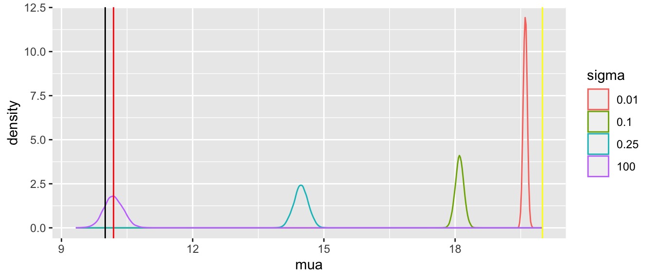
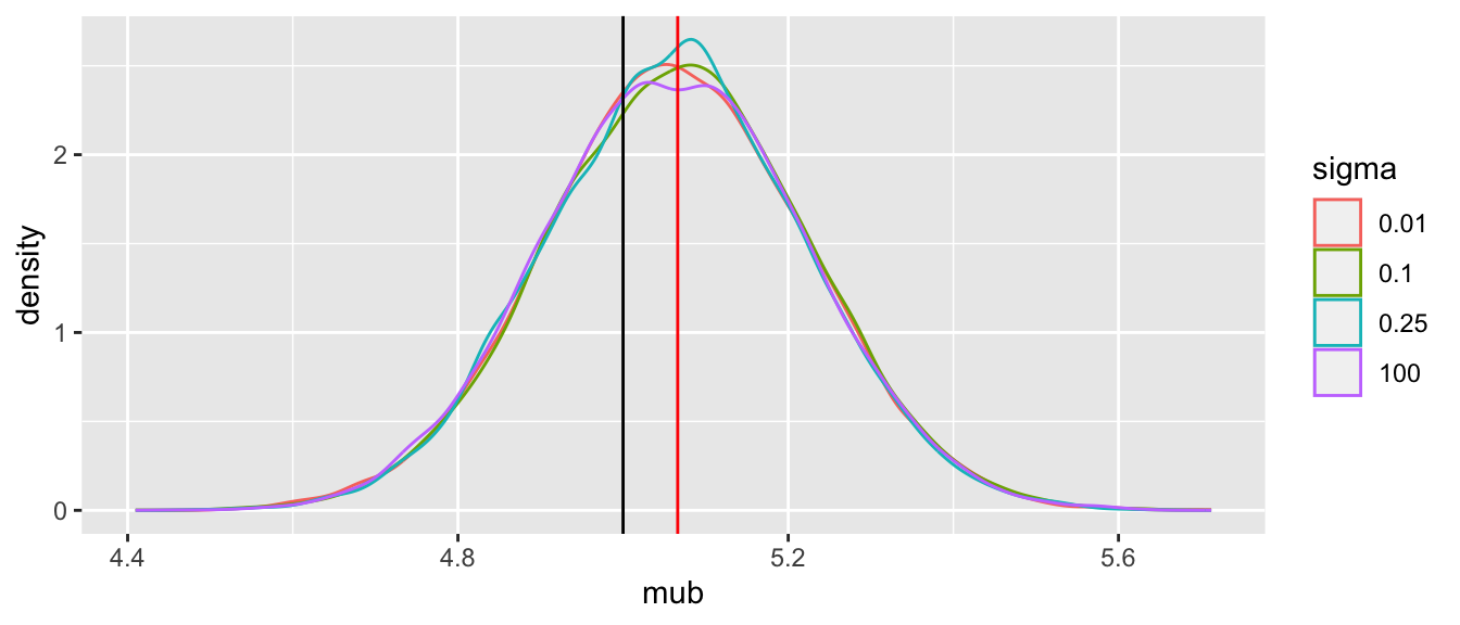
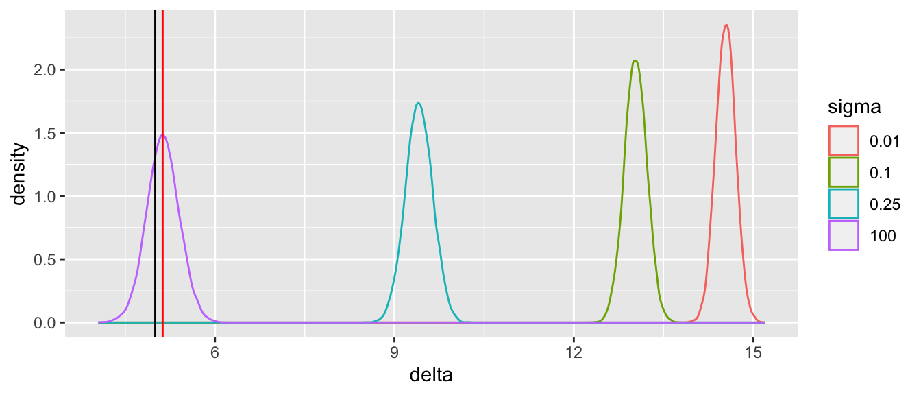
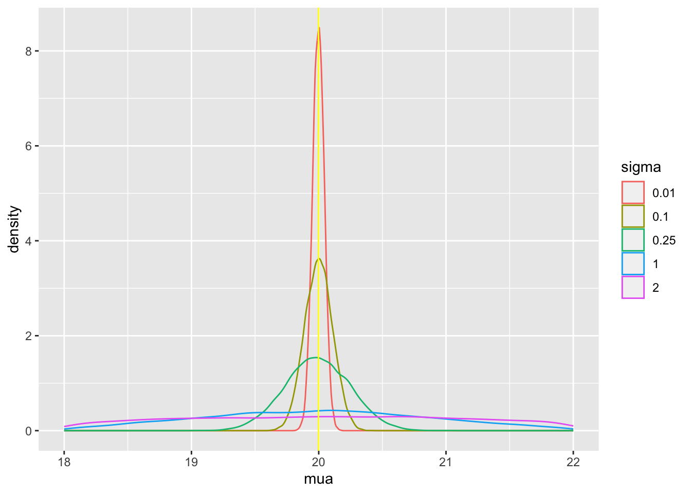
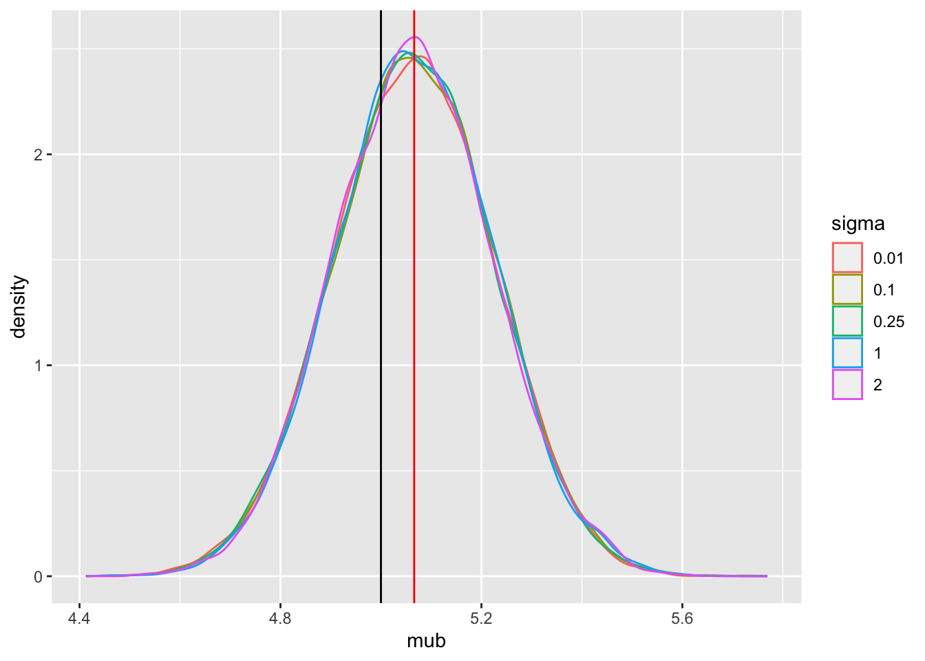
Tabular and graphical results follow. Black vertical lines indicate true values and red vertical lines indicate sample estimates from the RCT only. The yellow vertical line is the observed mean from HD.
Code
x <-rbind(g(sigma=100), g(sigma=0.01), g(sigma=0.1), g(sigma=0.25))
Note that the historical data does not inform the active treatment (B) estimates in any way. An SD of sigma=0.25 implies that the probability that the unknown bias is between -0.5 and 0.5 is 0.954.
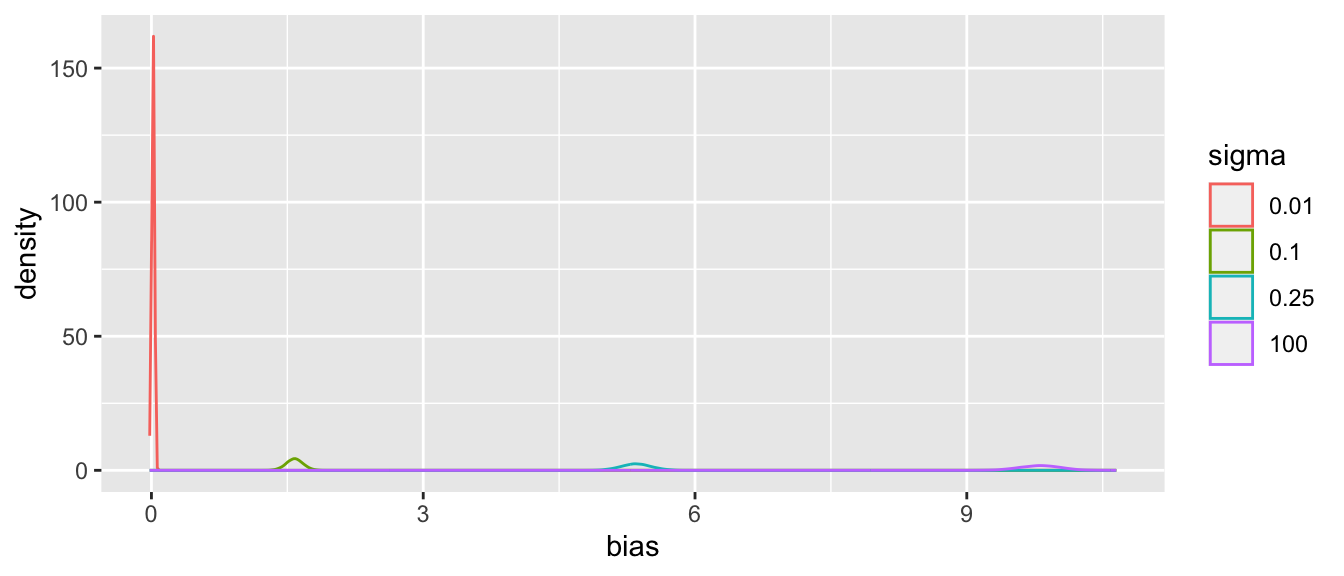
Posterior means and standard deviations, 0.05 and 0.95 quantiles (together making a 0.9 credible interval) and other quantities are shown in the tabular output above. When the prior belief about the bias of HD is encapsulated by sigma=0.01, i.e., HD are thought to be unbiased, the estimate mua of the true mean for treatment A (control) is very close to the observed mean of HD. When sigma=100 we know almost nothing about the applicability of HD and the posterior mean for A is almost identical to the sample mean in the trial. sigma=0.25 corresponds to the bias being possibly moderately large (since the raw data has SD=1.0), and the blended estimate of the true mean for A is larger than the RCT mean. We see corresponding changes in delta, the estimate of the A-B treatment effect. It is also of interest to examine the precision (narrowness of posterior distribution) when more information from HD bleeds over to the RCT.
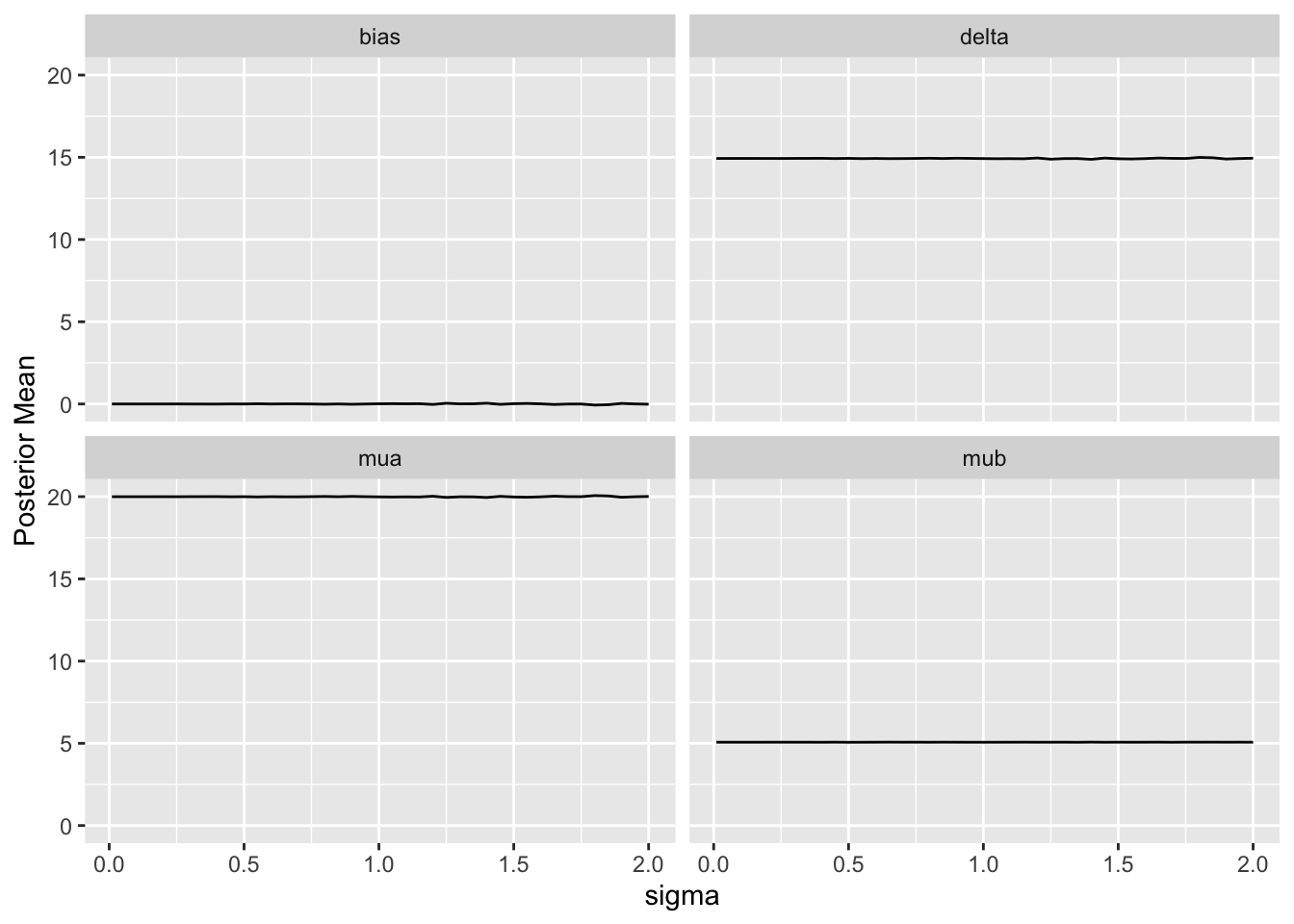
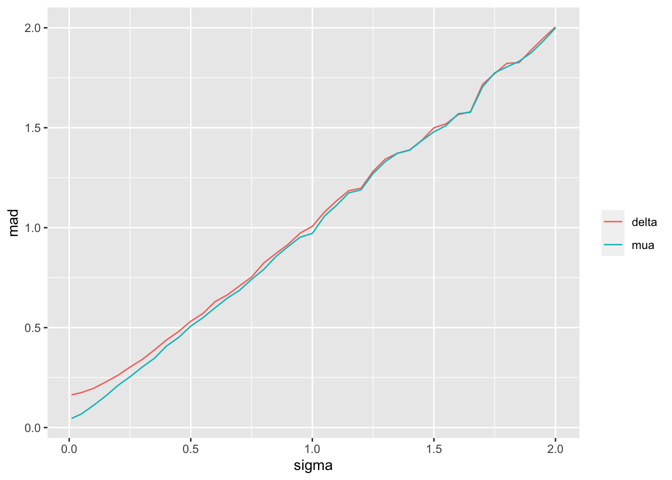
For a sequence of sigma values, plot how per-treatment posterior means, bias, and width of the posterior distribution (summarized by a mad mean absolute deviation measure) for the true mean of A vary. We are especially interested in how mad varies with increasing trust of HD.
Substantial information gain about the control mean mua and the treatment effect delta occur when sigma < 0.25. Of course in this simulation, any borrowing of HD is actually counterproductive because the HD mean violently disagrees with the treatment A sample mean.
Example: Creating a Control Arm With HD
What happens if the RCT is a single-arm trial trial and the control data come strictly from non-concurrent historical controls? In this case the bias in the HD cannot be estimated but will come solely from the assumed uncertainty distribution for the bias. The result is akin to a formal sensitivity analysis, but again the Bayesian paradigm provides a formal analysis tool that can easily be extended to include individual patient meta-analyses and covariate adjustment.
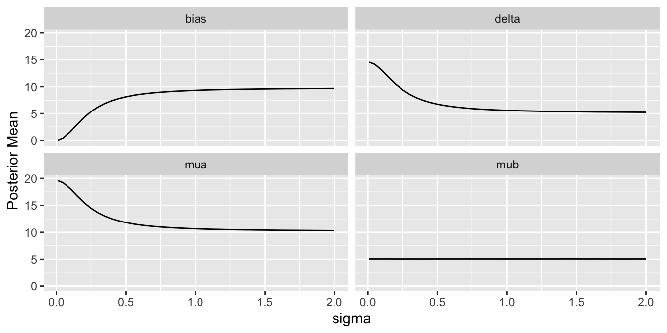
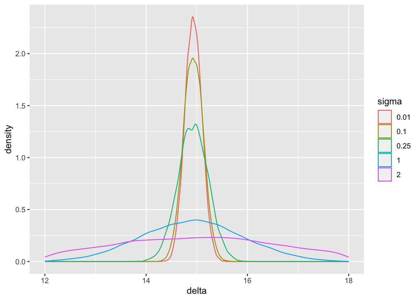
Let’s run examples similar to what was done for the augmented RCT control data but with only the single arm (treatment B) study data, and replacing the extreme sigma=100 case with sigma=1 and 2. A new Bayesian model is formulated to reflect that the HD were generated by a process having a mean that is the desired true mean mua plus an unknown bias.
Code
stancode2 <-'data { int<lower=0> Nb; // # obs in RCT treatment B int<lower=0> Nh; // # obs in historical control data vector[Nb] yb; // vector of tx=B data vector[Nh] yh; // vector of historical data real<lower=0> sigma; // standard deviation of prior for bias}parameters { real mua; // unknown mean for tx=A real mub; // unknown mean for tx=B real bias; // unknown bias}transformed parameters { real delta; delta = mua - mub;}model { yb ~ normal(mub, 1.0); yh ~ normal(mua + bias, 1.0); bias ~ normal(0., sigma);}'mod2 <-cmdstan_model(write_stan_file(stancode2))
The main parameter of interest is the treatment effect delta. The study is informative about delta if sigma < 2. For this simulation where the HD was generated to have an unrealistically high mean, we get misleading inference about delta if sigma is chosen to be \(\geq 2\). Note that for a response variable having a standard deviation of 1.0, 2.0 is an extremely large sigma.
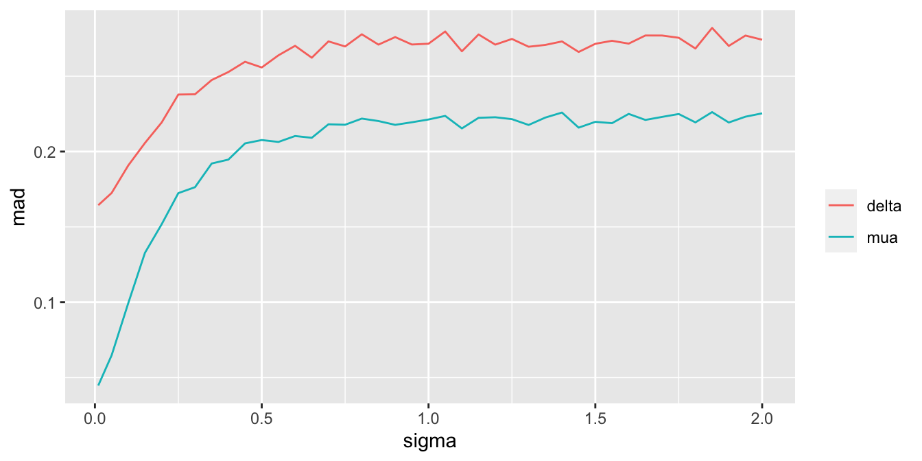
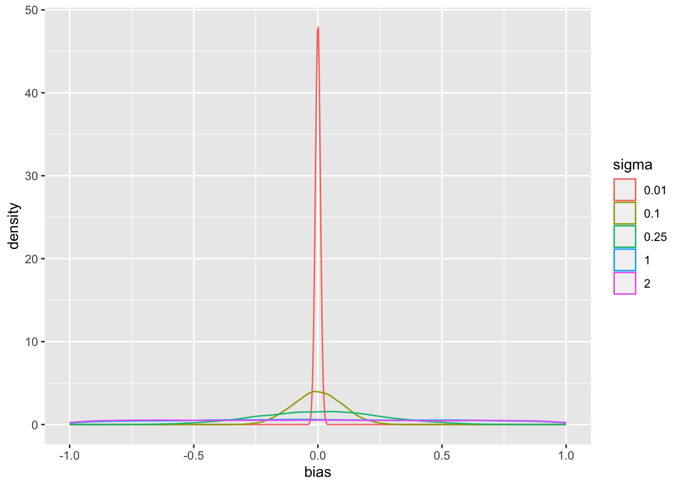
Since we assume that the bias is equally likely to be positive as negative (prior mean bias is zero which is also the posterior mean bias), sigma does not affect the posterior means of the parameters. It affects the width of the posterior distribution of mua and delta. The widths are summarized in the last plot above. When sigma=0, the HD are fully trusted as if they represent concurrent randomized control data.
Effective Sample Size
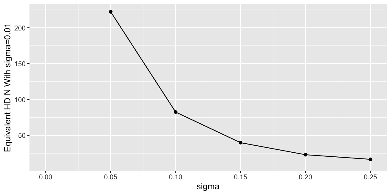
To get a sense of the effective sample sizes in estimating the control mean with different sigma, let’s summarize the posterior distribution width for mua using mad, and compare it to the mad under almost complete trust of HD (sigma=0.01). Vary the HD sample size Nh with sigma=0.01, compute mad, and use linear interpolation to solve for Nh that makes mad under a given sigma equal the mad under sigma=0.01.
Code
Nhs <-seq(10, 500, by=10)unlink('madn.rds')if(file.exists('madn.rds')) mads <-readRDS('madn.rds') else { f <-function(Nh) { d$yh <- yh[1: Nh] d$Nh <- Nh z <-g(sigma=0.01, raw=FALSE, model=mod2, data=d)subset(z, variable =='mua')$mad }sink('/tmp/z') mads <-sapply(Nhs, f)sink()saveRDS(mads, 'madn.rds')} s <-subset(stats2, variable =='mua')s$Neq <-approx(mads, Nhs, xout=s$mad)$yggplot(s, aes(x=sigma, y=Neq)) +geom_point() +geom_line() +ylab('Equivalent HD N With sigma=0.01') +xlim(0, 0.25)
Example Analytic Workflow
Consider the use of historical control HD for either a single investigational arm or two-arm RCT. Make the following assumptions for the present.
The same important covariates are present in both the RCT data and HD.
There are no covariate \(\times\) data source or covariate \(\times\) treatment interactions.
The bias from HD is equally likely to be negative as positive2.
The overall bias captures any secular trend resulting from the HD being out of date3.
2 If this is not the case, change the prior for the bias to something other than a Gaussian distribution with mean zero.
3 Otherwise, the secular trend will be confounded with the treatment effect.
Then develop an analytic plan along the following lines.
Select a fairly broad prior for the experimental treatment outcome tendency, unless there is a lot of prior clinical information that allows constraining this outcome tendency by knowledge of enrollment criteria.
Select a prior for the treatment effect with constraints based on what is known. If the treatment is a possible cure, contraints on differences in means, odds ratios, hazard ratios, etc., may be mild. If the therapy is incremental, it is appropriate to place a small prior probability on, say, the odds ratio being greater than 2 or less than 0.5.
Specify the prior distribution for bias based on what is known about evolution in therapy, patient selection bias, course of disease, etc. With the Bayesian analysis the exact amount of bias does not need to be known. Instead, the uncertainty distribution of bias must be specified. If this distribution is Gaussian, by the symmetry assumption mentioned earlier, what needs to be specified is the standard deviation \(\sigma\). This is best solved by specifying \(c\) such that \(\Pr(-c < \text{bias} < c) = 0.95\), for example, and backsolving for \(\sigma\)4.
Specify a realistic data model specifying treatment and covariate effects.
Including the model for bias at the point in the joint model where HD are used.
4 For example in a study to establish the effectiveness of a drug in lowering systolic blood pressure (SBP), one might choose \(\sigma\) for the bias in historical control mean SBP to be in a range of \(\pm 5\)mmHg with probability 0.95.
If either the RCT or HD data have any missing values for covariates, these can be handled in at least two ways:
Through joint modeling of outcomes and covariates, avoiding imputation
Through multiple imputation with multiple repeats of the Bayesian analyses, stacking all posterior draws into a single large matrix that is the basis for posterior probability calculations5.
5 Posterior stacking provides more accurate inference than Rubin’s rule with error degree of freedom adjustment in a frequentist analysis.
Summary
Bayesian joint modeling is a simple and natural way to model and penalize for potential bias from historical data. It is also extremely flexible in the kinds of HD that can be used, including mixtures of types of data. For example one could incorporate individual patient data meta analysis of a series of exchangeable studies, and data from a single study that was not exchangeable with the others. One could also borrow covariate effects across the RCT and HD, or allow each type of study to have its own covariate effects by including covariate interactions. It may be argued that direct modeling of bias is more realistic, and slightly less arbitrary, than choosing a prior that discounts all information from HD. By separating bias from variance, joint Bayesian models do not discount the HD sample size but instead discount what the HD is estimating. These models also lead to another type of generalization: modeling the bias as an increasing function of how long ago the historical data were collected.
---title: "Incorporating Historical Control Data Into an RCT"author: - name: Frank Harrell url: https://hbiostat.org affiliation: Department of Biostatistics<br>Vanderbilt University School of Medicinedate: 2023-11-04modified: 2023-12-27categories: [drug-evaluation, bayes, design, drug-development, inference, observational, posterior, prior, 2023]description: "Historical data (HD) are being used increasingly in Bayesian analyses when it is difficult to randomize enough patients to study effectiveness of a treatment. Such analyses summarize observational studies' posterior effectiveness distribution (for two-arm HD) or standard-of-care outcome distribution (for one-arm HD) then turn that into a prior distribution for an RCT. The prior distribution is then flattened somewhat to discount the HD. Since Bayesian modeling makes it easy to fit multiple models at once, incorporation of the raw HD into the RCT analysis and discounting HD by explicitly modeling bias is perhaps a more direct approach than lowering the effective sample size of HD. Trust the HD sample size but not what the HD is estimating, and realize several benefits from using raw HD in the RCT analysis instead of relying on HD summaries that may hide uncertainties."---## BackgroundIn studies of treatment effects for rare diseases, it is sometimes impossible to recruit enough patients to be able to randomize some of them to control therapy (e.g., standard of care). It other situations, it is difficult to recruit patients when they learn that half of them will not receive the new treatment. In pediatric drug studies, it may be easy to recruit adults into a randomized trial, but too few children may get the disease that is so prevalent in adults. In all these settings it may be desirable to borrow information from non-study patients. There are two major types of information to borrow. For pediatric studies, relative effectiveness of a drug in children can borrow information about relative effectiveness in adults. For other studies, historical data (HD) may be borrowed to provide or bolster the control arm in the RCT. For example, study leaders may wish to use 2:1 experimental : control randomization, but they know that there is a loss of precision and power from such an imbalance. Adding historical control information can make up for that if the HD are reliable and relevant enough.An area of highly active research in biostatistics is the choice of a prior distribution to properly discount HD for not being concurrent, for selection bias, and for other factors. One may take a posterior distribution from observational data and use discounting when incorporating it into a prior for the new study. For some procedures this amounts to lowering the effective sample size of the HD. This doesn't directly account for the bias from HD.An excellent background paper on historical controls is by [Schmidli _et al_](https://ascpt.onlinelibrary.wiley.com/doi/10.1002/cpt.1723). They discuss several ideas not covered here, including the need to adjust for differences in covariate distributions (including by matching on propensity scores). The approach outlined below readily extends to covariate adjustment if the same covariates used in the study are available in the raw HD. Missing values can be handled by adding more models to the joint Bayesian modeling process.What is presented here is related to the mean squared error (variance plus square of bias) of treatment effects estimated from observational data. A simulated example [here](https://www.fharrell.com/post/ehrs-rcts) shows how to compute the RCT sample size that will overcome the enhanced precision provided by larger observational studies that are biased.## Another ApproachConsider HD used to inform outcome tendencies in control patients.Rather than lowering the effective sample size of the HD, think about respecting the HD sample size but recognizing that the HD is estimating a different quantity than the actual prospective RCT control group outcome tendency. This different quantity is the true unknown control group performance plus the bias in the HD. This approach was proposed by [Stuart Pocock](https://www.sciencedirect.com/science/article/abs/pii/0021968176900448) in a frequentist context.[[Björn Holzhauer](https://www.tandfonline.com/doi/abs/10.1080/19466315.2019.1610043) developed related Bayesian approaches for borrowing exponential hazard rates from HD.]{.aside}Now couple that idea with another one. In trying to specify a posterior distribution from an HD analysis to be fed into a prior for the new study, the same goal may be accomplished by noting that Bayesian MCMC simulation procedures (to obtain posterior samples of the parameters of interest) allow multiple models to be processed simultaneously. This is especially the case with [Stan](https://mc-stan.org). The information from HD can be incorporated into the new analysis by actually specifying a model for the HD and bringing the HD raw data into the analysis of the new trial data. Next, when forming the second model (for HD), explicitly model the possibility that HD are estimating a different estimand than the RCT. When the HD being used consist solely of control patient data, this different estimand is the true unknown outcome measure for randomized concurrent control patients, plus an unknown bias.There is subtle and important ramification of the approach of merging multiple raw data streams and distinguishing the data source by having multiple models being fitted simultaneously. Most applications of data borrowing oversimplify the data being borrowed. For example, researchers often use summary statistics from historical data including standard errors (SEs). SEs are only estimates of precision of parameter estimates, and treating the SEs as if they are calculated without error is ignoring important uncertainty, giving false confidence in the historical data. By including raw HD in the RCT analysis, all uncertainties are accounted for, making final Bayesian uncertainty intervals properly wider to avoid false confidence. On a related note, when there is important within-treatment outcome heterogeneity necessitating the use of covariate adjustment in both non-randomized and randomized data, researchers very frequently make the mistake of using marginal treatment effect summaries of the HD. In nonlinear models (e.g., Cox and logistic models) estimated treatment effects are [shrunken towards the null](https://hbiostat.org/bbr/ancova) by the unexplained outcome heterogeneity (caused by wide covariate distributions) that could have been easily explained through direct covariate adjustment^[Suppose that sex is an important prognostic factor. Ignoring sex when comparing treatments may make a within-treatment outcome distribution become a mixture of two distributions and even be bimodal, and make a treatment that operates in proportional hazards for both males and females separately not act in proportional hazards when indiscriminately pooling males and females.]. Incorporation of raw HD allows for proper covariate adjustment. The same covariate adjustment also balances the playing field with regard to differences in covariate distributions between RCT and HD. Instead of discarding data using propensity matching of RCT to HD to account for, say, patients in the HD being older, age can be directly adjusted for in a much more efficient exclude-no-data approach.For the examples that follow, we assume that no data are available for estimating the bias, and that bias is described by a prior distribution that is Gaussian with a mean bias of zero and with a standard deviation of `sigma`. When `sigma` is zero, the bias is known to be exactly zero, and the HD are pooled with any study control data, with full weight given to HD. When `sigma` is $\infty$, we know nothing at all about bias, and HD are non-informative and effectively ignored.## Example: Augmenting a Control Arm with HDLet's see how this plays out with several choices of `sigma`. First let's get access to the needed R packages including `cmdstanr` which uses `Command Stan`, and specify the Stan modeling code we need to get the posterior draws from our two-model system. The key idea in the code below is the model for the HD `yh` which is `yh ~ normal(mua + bias, 1.0)`. The historical data for treatment A are connected to the RCT data by the `yh` model having the parameter `mua` in common with the RCT control arm. The two are also disconnected by having the `bias` parameter added to the mean model for `yh`. So `mua` is estimated by combining study data and HD after de-biasing HD.```{r}require(cmdstanr)# set_cmdstan_path('/usr/local/bin/cmdstan-2.33.1')require(ggplot2)options(mc.cores=4) # each chain run on a separate CPUstancode <-'data { int<lower=0> Na; // # obs in RCT treatment A (control) int<lower=0> Nb; // # obs in RCT treatment B int<lower=0> Nh; // # obs in historical control data vector[Na] ya; // vector of tx=A data vector[Nb] yb; // vector of tx=B data vector[Nh] yh; // vector of historical data real<lower=0> sigma; // standard deviation of prior for bias}parameters { real mua; // unknown mean for tx=A real mub; // unknown mean for tx=B real bias; // unknown bias}transformed parameters { real delta; delta = mua - mub;}model { ya ~ normal(mua, 1.0); yb ~ normal(mub, 1.0); yh ~ normal(mua + bias, 1.0); bias ~ normal(0., sigma);}'mod <-cmdstan_model(write_stan_file(stancode))```Next simulate the normally distributed data we'll analyze, from a 2:1 B:A randomization with 20 patients in arm A (control) and 40 in arm B. HD are available on 500 patients. The raw data are assumed to have standard deviation of 1.0. The true mean for A is 10, the mean for B is 5, and the HD are very biased with a mean of 20 instead of the target of 10. An extreme bias is used here just for illustration, to make results stand out. The simulation can easily be run with other settings.```{r}set.seed(1)Na <-20Nb <-40Nh <-500ya <-rnorm(Na, 10)yb <-rnorm(Nb, 5)yh <-rnorm(Nh, 20)cat('Sample means:\n')round(c(a=mean(ya), b=mean(yb), h=mean(yh), bias=mean(yh)-mean(ya)), 2)d <-list(Na=Na, Nb=Nb, Nh=Nh, ya=ya, yb=yb, yh=yh)```Next run Bayesian analyses separately for each of four `sigma` values.```{r}# Write a little function that runs cmdstan to get posterior draws,# print posterior summaries and MCMC diagnostics, and save the# draws in a data frame if raw=TRUE. Otherwise save summary stats.g <-function(sigma, raw=TRUE, model=mod, data=d) { data$sigma <- sigma f <- model$sample(data=data, seed=3, chains=4, refresh=0,iter_warmup=500, iter_sampling=4000)if(! raw) { s <- f$summary(variables=c('mua', 'mub', 'delta', 'bias'))[, c('variable', 'mean', 'mad')] s <-data.frame(s) s$sigma <- sigmareturn(s) }cat('\n--------------------------------\nsigma=', sigma,'\n--------------------------------\n')print(f$summary()) x <- f$draws(c('mua', 'mub', 'delta', 'bias'), format='df') x$sigma <- sigma x}```Tabular and graphical results follow. Black vertical lines indicate true values and red vertical lines indicate sample estimates from the RCT only. The yellow vertical line is the observed mean from HD.```{r}#| fig-height: 3x <-rbind(g(sigma=100), g(sigma=0.01), g(sigma=0.1), g(sigma=0.25))pdens <-function(mualim=NULL, deltalim=NULL, biaslim=NULL) { x$sigma <-factor(x$sigma) g1 <-ggplot(x, aes(x=mua, color=sigma)) +geom_density() +geom_vline(xintercept=10) +geom_vline(xintercept=mean(ya), col=I('red')) +geom_vline(xintercept=mean(yh), col=I('yellow'))if(length(mualim)) g1 <- g1 +xlim(mualim) g2 <-ggplot(x, aes(x=mub, color=sigma)) +geom_density() +geom_vline(xintercept=5) +geom_vline(xintercept=mean(yb), col=I('red')) g3 <-ggplot(x, aes(x=delta, color=sigma)) +geom_density() +geom_vline(xintercept=5) +geom_vline(xintercept=mean(ya) -mean(yb), col=I('red'))if(length(deltalim)) g3 <- g3 +xlim(deltalim) g4 <-ggplot(x, aes(x=bias, color=sigma)) +geom_density()if(length(biaslim)) g4 <- g4 +xlim(biaslim)print(g1); print(g2); print(g3); print(g4)invisible()}pdens()```Note that the historical data does not inform the active treatment (B) estimates in any way.An SD of `sigma`=0.25 implies that the probability that the unknown bias is between -0.5 and 0.5 is `r round(pnorm(0.5, sd=0.25) - pnorm(-0.5, sd=0.25), 3)`.Posterior means and standard deviations, 0.05 and 0.95 quantiles (together making a 0.9 credible interval) and other quantities are shown in the tabular output above. When the prior belief about the bias of HD is encapsulated by `sigma`=0.01, i.e., HD are thought to be unbiased, the estimate `mua` of the true mean for treatment A (control) is very close to the observed mean of HD. When `sigma`=100 we know almost nothing about the applicability of HD and the posterior mean for A is almost identical to the sample mean in the trial. `sigma`=0.25 corresponds to the bias being possibly moderately large (since the raw data has SD=1.0), and the blended estimate of the true mean for A is larger than the RCT mean. We see corresponding changes in `delta`, the estimate of the A-B treatment effect. It is also of interest to examine the precision (narrowness of posterior distribution) when more information from HD bleeds over to the RCT.For a sequence of `sigma` values, plot how per-treatment posterior means, bias, and width of the posterior distribution (summarized by a `mad` mean absolute deviation measure) for the true mean of A vary. We are especially interested in how `mad` varies with increasing trust of HD.```{r}#| fig-height: 3.5sigmas <-pmax(0.01, seq(0, 2, by=0.05))if(file.exists('stats.rds')) stats <-readRDS('stats.rds') else {sink('/tmp/z') stats <-do.call('rbind', lapply(sigmas, g, raw=FALSE))saveRDS(stats, 'stats.rds')sink()}ptrend <-function(s) { g1 <-ggplot(s, aes(x=sigma, y=mean)) +geom_line() +facet_wrap(~ variable) +ylab('Posterior Mean') g2 <-ggplot(subset(s, variable %in%c('mua', 'delta')),aes(x=sigma, y=mad, color=variable)) +geom_line() +guides(color=guide_legend(title=''))print(g1); print(g2)invisible()}ptrend(stats)```Substantial information gain about the control mean `mua` and the treatment effect `delta` occur when `sigma` < 0.25. Of course in this simulation, any borrowing of HD is actually counterproductive because the HD mean violently disagrees with the treatment A sample mean.## Example: Creating a Control Arm With HDWhat happens if the RCT is a single-arm trial trial and the control data come strictly from non-concurrent historical controls? In this case the bias in the HD cannot be estimated but will come solely from the assumed uncertainty distribution for the bias. The result is akin to a formal sensitivity analysis, but again the Bayesian paradigm provides a formal analysis tool that can easily be extended to include individual patient meta-analyses and covariate adjustment.Let's run examples similar to what was done for the augmented RCT control data but with only the single arm (treatment B) study data, and replacing the extreme `sigma`=100 case with `sigma`=1 and 2. A new Bayesian model is formulated to reflect that the HD were generated by a process having a mean that is the desired true mean `mua` plus an unknown `bias`.```{r}stancode2 <-'data { int<lower=0> Nb; // # obs in RCT treatment B int<lower=0> Nh; // # obs in historical control data vector[Nb] yb; // vector of tx=B data vector[Nh] yh; // vector of historical data real<lower=0> sigma; // standard deviation of prior for bias}parameters { real mua; // unknown mean for tx=A real mub; // unknown mean for tx=B real bias; // unknown bias}transformed parameters { real delta; delta = mua - mub;}model { yb ~ normal(mub, 1.0); yh ~ normal(mua + bias, 1.0); bias ~ normal(0., sigma);}'mod2 <-cmdstan_model(write_stan_file(stancode2))``````{r}d$Na <- d$ya <-NULL# remove RCT control armx <-rbind(g(sigma=2, model=mod2), g(sigma=1, model=mod2),g(sigma=0.01, model=mod2),g(sigma=0.1, model=mod2), g(sigma=0.25, model=mod2))pdens(mualim=c(18,22), deltalim=c(12,18), biaslim=c(-1, 1))```The main parameter of interest is the treatment effect `delta`. The study is informative about `delta` if `sigma` < 2. For this simulation where the HD was generated to have an unrealistically high mean, we get misleading inference about `delta` if `sigma` is chosen to be $\geq 2$. Note that for a response variable having a standard deviation of 1.0, 2.0 is an extremely large `sigma`.```{r}if(file.exists('stats2.rds')) stats2 <-readRDS('stats2.rds') else {sink('/tmp/z') stats2 <-do.call('rbind', lapply(sigmas, g, raw=FALSE, model=mod2))saveRDS(stats2, 'stats2.rds')sink()}ptrend(stats2)```Since we assume that the bias is equally likely to be positive as negative (prior mean `bias` is zero which is also the posterior mean `bias`), `sigma` does not affect the posterior means of the parameters. It affects the width of the posterior distribution of `mua` and `delta`. The widths are summarized in the last plot above. When `sigma`=0, the HD are fully trusted as if they represent concurrent randomized control data.### Effective Sample SizeTo get a sense of the effective sample sizes in estimating the control mean with different `sigma`, let's summarize the posterior distribution width for `mua` using `mad`, and compare it to the `mad` under almost complete trust of HD (`sigma`=0.01). Vary the HD sample size `Nh` with `sigma`=0.01, compute `mad`, and use linear interpolation to solve for `Nh` that makes `mad` under a given `sigma` equal the `mad` under `sigma`=0.01.```{r}#| fig-height: 3.5Nhs <-seq(10, 500, by=10)unlink('madn.rds')if(file.exists('madn.rds')) mads <-readRDS('madn.rds') else { f <-function(Nh) { d$yh <- yh[1: Nh] d$Nh <- Nh z <-g(sigma=0.01, raw=FALSE, model=mod2, data=d)subset(z, variable =='mua')$mad }sink('/tmp/z') mads <-sapply(Nhs, f)sink()saveRDS(mads, 'madn.rds')} s <-subset(stats2, variable =='mua')s$Neq <-approx(mads, Nhs, xout=s$mad)$yggplot(s, aes(x=sigma, y=Neq)) +geom_point() +geom_line() +ylab('Equivalent HD N With sigma=0.01') +xlim(0, 0.25)```## Example Analytic WorkflowConsider the use of historical control HD for either a single investigational arm or two-arm RCT. Make the following assumptions for the present.1. The same important covariates are present in both the RCT data and HD.1. There are no covariate $\times$ data source or covariate $\times$ treatment interactions.1. The bias from HD is equally likely to be negative as positive^[If this is not the case, change the prior for the bias to something other than a Gaussian distribution with mean zero.].1. The overall bias captures any secular trend resulting from the HD being out of date^[Otherwise, the secular trend will be confounded with the treatment effect.].Then develop an analytic plan along the following lines.1. Select a fairly broad prior for the experimental treatment outcome tendency, unless there is a lot of prior clinical information that allows constraining this outcome tendency by knowledge of enrollment criteria.1. Select a prior for the treatment effect with constraints based on what is known. If the treatment is a possible cure, contraints on differences in means, odds ratios, hazard ratios, etc., may be mild. If the therapy is incremental, it is appropriate to place a small prior probability on, say, the odds ratio being greater than 2 or less than 0.5.1. Specify the prior distribution for bias based on what is known about evolution in therapy, patient selection bias, course of disease, etc. With the Bayesian analysis the exact _amount_ of bias does not need to be known. Instead, the _uncertainty distribution_ of bias must be specified. If this distribution is Gaussian, by the symmetry assumption mentioned earlier, what needs to be specified is the standard deviation $\sigma$. This is best solved by specifying $c$ such that $\Pr(-c < \text{bias} < c) = 0.95$, for example, and backsolving for $\sigma$^[For example in a study to establish the effectiveness of a drug in lowering systolic blood pressure (SBP), one might choose $\sigma$ for the bias in historical control mean SBP to be in a range of $\pm 5$mmHg with probability 0.95.].1. Specify a realistic data model specifying treatment and covariate effects.1. Including the model for bias at the point in the joint model where HD are used.If either the RCT or HD data have any missing values for covariates, these can be handled in at least two ways:* Through joint modeling of outcomes and covariates, avoiding imputation* Through multiple imputation with multiple repeats of the Bayesian analyses, stacking all posterior draws into a single large matrix that is the basis for posterior probability calculations^[Posterior stacking provides more accurate inference than Rubin's rule with error degree of freedom adjustment in a frequentist analysis.].## SummaryBayesian joint modeling is a simple and natural way to model and penalize for potential bias from historical data. It is also extremely flexible in the kinds of HD that can be used, including mixtures of types of data. For example one could incorporate individual patient data meta analysis of a series of exchangeable studies, and data from a single study that was not exchangeable with the others. One could also borrow covariate effects across the RCT and HD, or allow each type of study to have its own covariate effects by including covariate interactions. It may be argued that direct modeling of bias is more realistic, and slightly less arbitrary, than choosing a prior that discounts all information from HD. By separating bias from variance, joint Bayesian models do not discount the HD sample size but instead discount what the HD is estimating. These models also lead to another type of generalization: modeling the bias as an increasing function of how long ago the historical data were collected.---* [Discussion board](https://discourse.mc-stan.org/t/blog-article-on-bayesian-thinking-in-the-use-of-historical-control-data)---## Resources * [Applying Quantitative Bias Analysis to Epidemiologic Data](https://link.springer.com/book/10.1007/978-3-030-82673-4) by MP Fox, RF MacLehose, TL Lash * [Multiple-bias modelling for analysis of observational data](https://rss.onlinelibrary.wiley.com/doi/abs/10.1111/j.1467-985X.2004.00349.x) by S Greenland**Acknowledgements**Thanks to Björn Holzhauer, Bob Carpenter, and Andrew Gelman for their valuable input.