It is well known that the score test for comparing survival distributions between two groups without covariate adjustment, using a Cox proportional hazards (PH) model, is identical to the log-rank \(\chi^2\) test when there are no tied failure times. Yet there persists a belief that the log-rank test is somehow completely nonparametric and does not assume PH. Log-rank and Cox approaches can only disagree if the more commonly used likelihood ratio (LR) statistic from the Cox model disagrees with the log-rank statistic (and the Cox score statistic). This article shows that in fact the log-rank and Cox LR statistics agree to a remarkable degree, and furthermore the hazard ratio arising from the log-rank test also has remarkable agreement with the Cox model counterpart. Since both methods assume PH and the log-rank test assumes within-group heterogeneity (because it doesn’t allow for covariate adjustment), the Cox model actually makes fewer assumptions than log-rank.
Department of Biostatistics Vanderbilt University School of Medicine
Published
March 28, 2024
Modified
March 31, 2024
Background
The log-rank test is a Mantel-Haenszel “observed - expected frequency” type of test that was derived in a slightly ad hoc way by Nathan Mantel in 1966 and named the logrank test by R Peto and J Peto in 1972. It was later formally derived as the rank test having optimal local power for a shift in the type I extreme value (Gumbel) distribution. This horizontal shift is equivalent to a vertical shift in survival distributions after log-log transforming them. This is identical to saying the two survival distributions are in proportional hazards, i.e., that one survival curve is the other one raised to a constant power.
It is well known that when a Cox proportional hazards (PH) model contains only a single covariate, and it is binary, this two-group-comparison setup gives rise to a Rao score test1 for testing the difference between the two groups. This score test is identical to the log-rank test statistic when there are no ties in the failure times. So we already know that the log-rank test makes all the assumptions of a Cox PH model, and in a sense we can go further than that. The two approaches are one and the same when there are only groups and no covariates.
1 The score test has in the numerator the first derivative of the Cox log-likelihood function with respect to the regression coefficient \(\beta\), evaluated at \(\beta=0\).
Therefore the only question that is unsettled relates to the fact that the score test is not used very frequently with the Cox model, opting for the Wald statistic or the gold-standard likelihood ratio (LR) statistic. This article uses simulated datasets to show how little it matters when one compares the log-rank statistic with the Cox LR instead of the score statistic. I also show that the Pike log-rank HR estimate agrees extremely well with the Cox HR estimate.
There are two HRs that go along with the log-rank test, the Pike estimator and the Peto estimator. The linked article shows that the Pike HR estimator is better. This HR estimator is the ratio of two ratios. Each of these ratios is the ratio of the observed number of events in a group to the expected number of events in the group.
See this article for more about the log-rank test and the difference between semiparametric and truly nonparametric assumption-free methods.
Simulated Numerical Examples
Fast code for computing the two-sample log-rank \(\chi^2\) statistic and the Pike HR is found in the Hmisc package:
function (S, group)
{
    i <- is.na(S) | is.na(group)
    if (any(i)) {
        i <- !i
        S <- S[i, , drop = FALSE]
        group <- group[i]
    }
    u <- sort(unique(group))
    if (length(u) > 2)
        stop("group must have only 2 distinct values")
    x <- ifelse(group == u[2], 1, 0)
    y <- S[, 1]
    event <- S[, 2]
    i <- order(-y)
    y <- y[i]
    event <- event[i]
    x <- x[i]
    x <- cbind(1 - x, x, (1 - x) * event, x * event)
    s <- rowsum(x, y, FALSE)
    nr1 <- cumsum(s[, 1])
    nr2 <- cumsum(s[, 2])
    d1 <- s[, 3]
    d2 <- s[, 4]
    rd <- d1 + d2
    rs <- nr1 + nr2 - rd
    n <- nr1 + nr2
    oecum <- d1 - rd * nr1/n
    vcum <- rd * rs * nr1 * nr2/n/n/(n - 1)
    chisq <- sum(oecum)^2/sum(vcum, na.rm = TRUE)
    o1 <- sum(d1)
    o2 <- sum(d2)
    e1 <- sum(nr1 * rd/n)
    e2 <- sum(nr2 * rd/n)
    hr <- (o2/e2)/(o1/e1)
    structure(chisq, hr = hr)
}
<bytecode: 0x11bdf73b8>
<environment: namespace:Hmisc>
The likelihood ratio, score, and Wald statistics for the Cox model are computed by the survival package’s coxph function.
To compare Cox and log-rank statistics empirically we can create a large number of datasets with two groups and some observations right-censored. With enough randomness, both PH and a variety of non-PH are achieved.
Here is a function to simulate one dataset with n total observations. The data generating mechanism has PH in play since group is ignored, but with a sufficient number of random datasets generated the data patterns will cover all sorts of non-PH and strengths of the group effect. The simulations are for a sample size of \(n=40\) with the fraction of observations in the first group randomly varying from \(\frac{n}{4}\) to \(\frac{n}{2}\). The fraction of right-censored observations varies randomly from 0.1 to 0.9. Failure times have a uniform distribution.
Code
sim1 <-function(n=40) {# Specific sample size for group 1, uniformly between# n/4 and n/2 n1 <-sample(round(c(n /4, n /2)), 1) n2 <- n - n1 x <-c(rep(0, n1), rep(1, n2)) y <-runif(n)# Proportion of right-censoring ranges from 0.1 to 0.9 uniformly cprop <-runif(1, 0.1, 0.9) ev <-ifelse(runif(n) < cprop, 0, 1) S <-Surv(y, ev)data.frame(x, S)}
log-rank \(\chi^{2} \equiv\) Cox Score Test
First check exact agreement between log-rank and Cox score statistics on 10 random datasets so that we don’t need to compute both of them.
Simulated Trials with \(n=40\) To Compare HR and LR
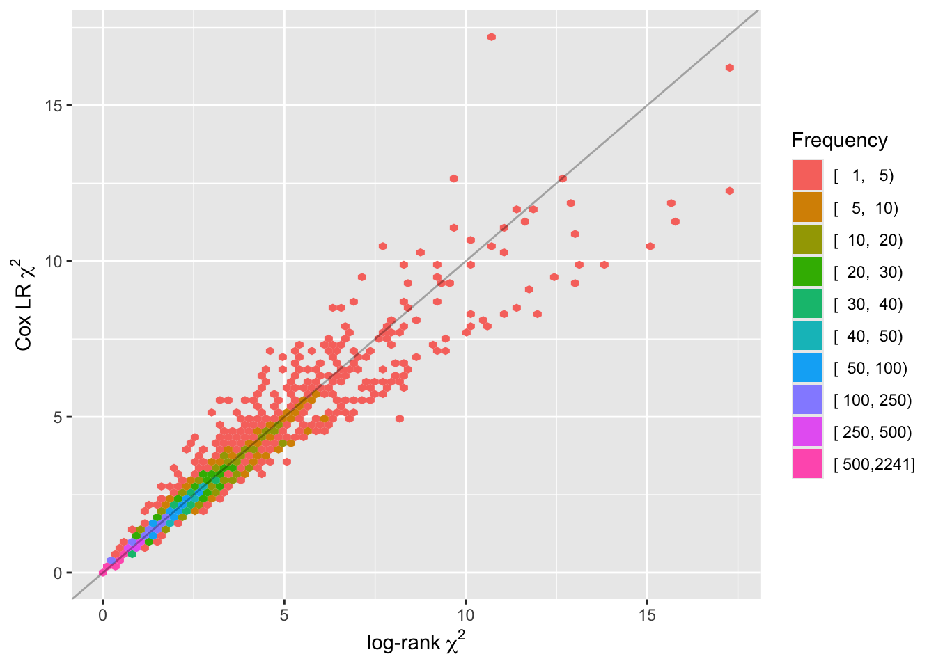
Now simulate a large number of trials with \(n=40\), and save the log-rank and its associated hazard ratio (HR) estimate, and the Cox model likelihood ratio \(\chi^2\) and its maximum likelihood estimate of the HR.
The hexagonal binning plot with color-coded bin frequencies shows amazing agreement between log-rank and Cox LR. Most of the \(\chi^2\) in the simulated datasets are between 0 and 5 and fall right on the line of identity.
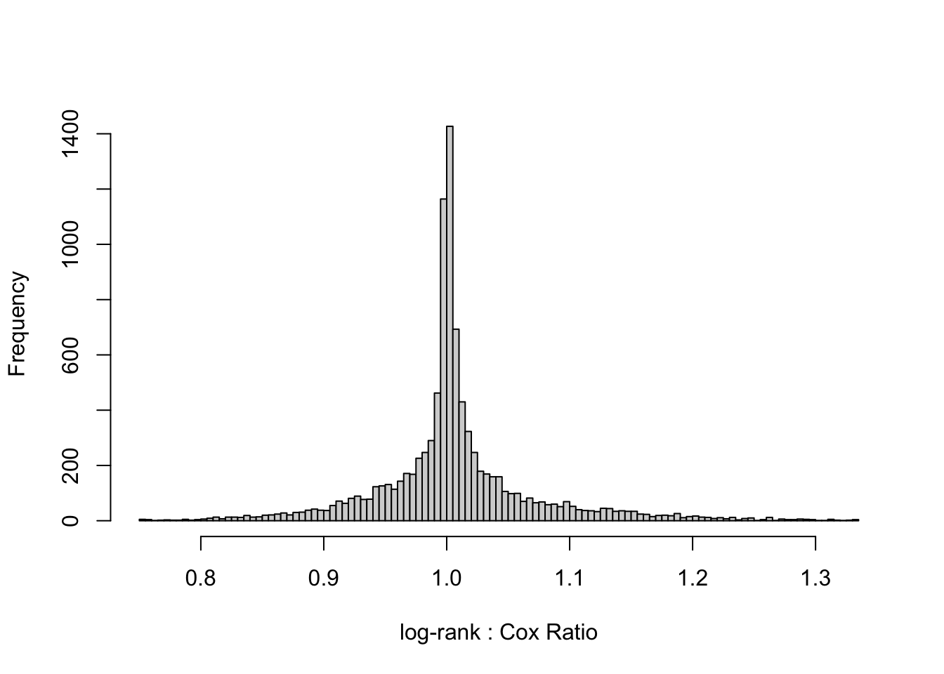
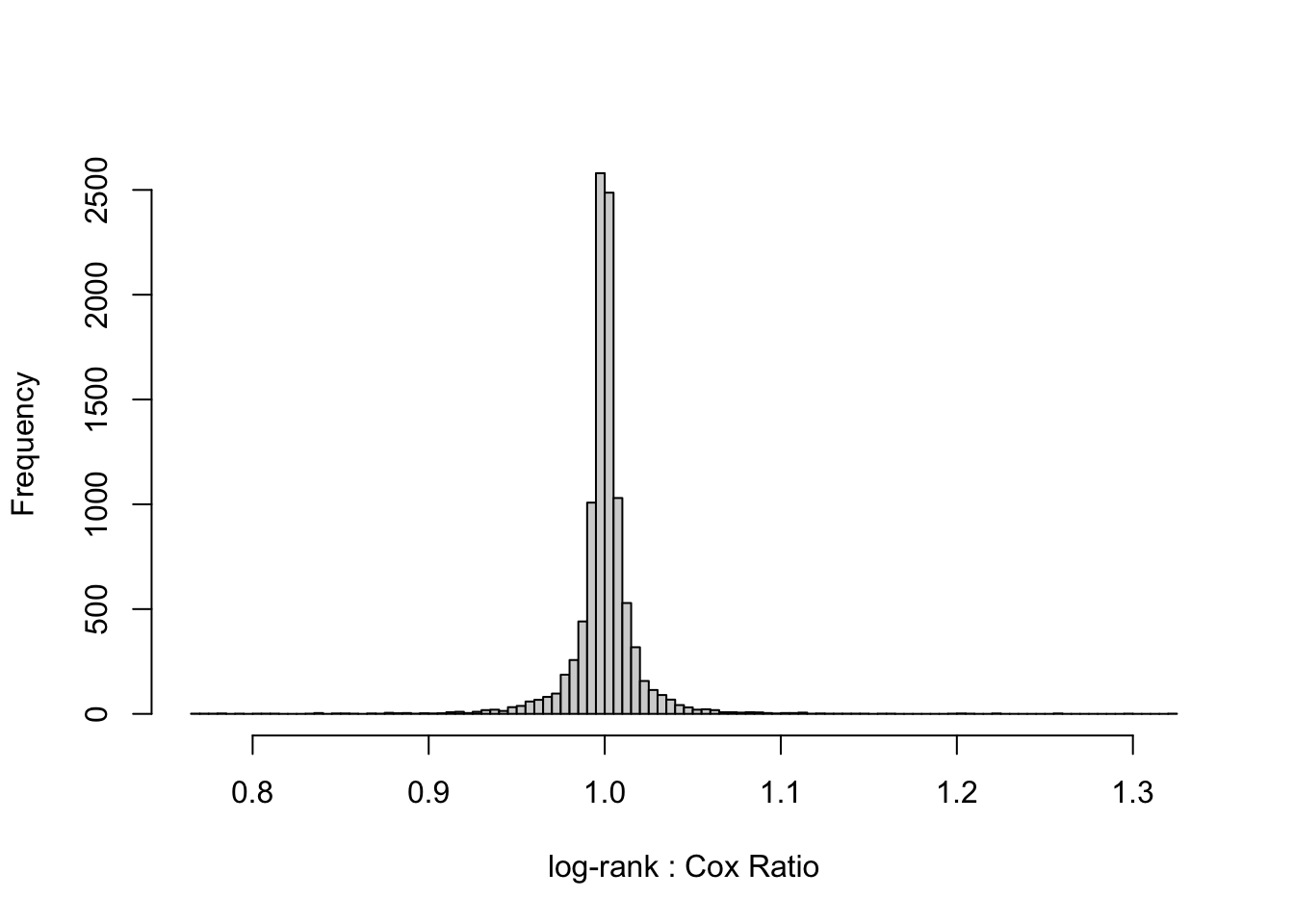
Estimate the typical ratio of the two \(\chi^2\), and the Spearman \(\rho\) rank correlation between them over datasets. Also show quantiles of the ratios of the two \(\chi^2\).
Code
# Function to compute Spearman's rank correlation coefficient# and fold-change discrepancy# Also prints quantiles of ratios and plots histogram of ratioss <-function(x, y, pl=TRUE) { rho <-cor(x, y, method='spearman') ratio <- x / y qu <-quantile(ratio, c(.01, .05, .1, .25, .5, .75, .9, .95, .99))cat('Quantiles of ratios of log-rank statistic to Cox statistic\n\n')print(round(qu, 3))hist(ratio[ratio >0.75& ratio <1/0.75], nclass=100,main='', xlab='log-rank : Cox Ratio') fc <-exp(median(abs(log(ratio))))list(rho=round(rho, 3), fold_change=round(fc, 3))}dchi <- w[, s(logrank, lr)]
Quantiles of ratios of log-rank statistic to Cox statistic

   1%    5%   10%   25%   50%   75%   90%   95%   99%
0.812 0.900 0.936 0.984 1.001 1.021 1.083 1.135 1.242
Code
dchi
     rho fold_change
1: 0.999       1.019
The typical (median) multiplicative (fold change) discrepancy between the log-rank \(\chi^2\) and the Cox LR \(\chi^2\) is a ratio of 1.019, and the Spearman rank correlation between the two test statistics over the 10,000 random datasets with \(n=40\) is 0.999. The two test statistics tend to agree to within a factor of 1.019.
See how often the two test statistics agree on being near zero.
Code
w[, table(logrank <0.001, lr <0.001)]
        FALSE TRUE
  FALSE  9558    0
  TRUE      0  241
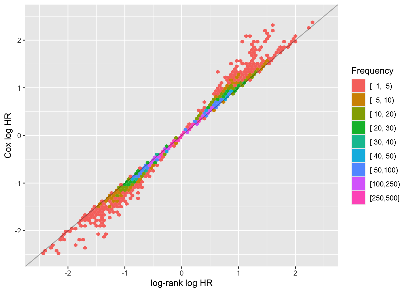
Perfect agreement. Now examine agreement in estimated HRs.
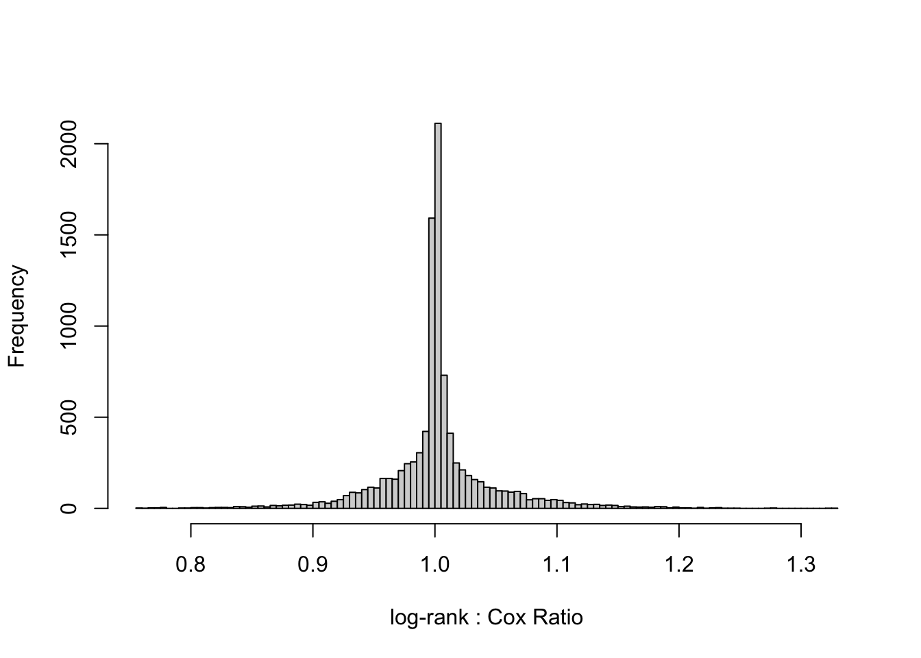
Quantiles of ratios of log-rank statistic to Cox statistic

   1%    5%   10%   25%   50%   75%   90%   95%   99%
0.762 0.917 0.956 0.987 1.000 1.016 1.048 1.088 1.253
Code
dhr
     rho fold_change
1: 0.999       1.014
Again, the scatter plot shows tremendous agreement between the log-rank and Cox model. The median fold change discrepancy between the log-rank HR and the Cox partial maximum likelihood estimated HR is 1.014, and the Spearman rank correlation between the two HRs over the 10,000 random datasets with \(n=40\) is 0.999.
When the Pike log-rank HR is zero, compute the maximum Cox HR. When the Pike HR is zero, the Cox HR is \(< 10^{-9}\).
Code
w[logrankHR ==0, signif(max(coxHR), 3)]
[1] 1.06e-09
Here is the frequency distribution of the Pike HR when the Cox HR is \(< 10^{-9}\).
Now repeat some of this for \(n=100\). The agreement between Cox and log-rank gets better the larger the sample size.
Code
u <-data.table(i =1: nsim)u <- u[, g(n=100), by=i] # 13s for 10,000 studiescat('Agreement on chi-square\n\n')
Agreement on chi-square
Code
u[, s(logrank, lr, pl=FALSE)]
Quantiles of ratios of log-rank statistic to Cox statistic

   1%    5%   10%   25%   50%   75%   90%   95%   99%
0.852 0.930 0.955 0.990 1.000 1.011 1.052 1.085 1.154
   rho fold_change
1:   1       1.011
Code
cat('Agreement on HR\n\n')
Agreement on HR
Code
u[, s(logrankHR, coxHR, pl=FALSE)]
Quantiles of ratios of log-rank statistic to Cox statistic

   1%    5%   10%   25%   50%   75%   90%   95%   99%
0.935 0.975 0.986 0.995 1.000 1.005 1.015 1.025 1.063
   rho fold_change
1:   1       1.005
Summary
The log-rank statistic and its associated hazard ratio estimator both assume proportional hazards to the same degree, because the numerical values of the statistics (both \(\chi^2\) and HR) agree exceptionally well no matter what data patterns exist. This is for the case where two groups are being compared, and there is within-group homogeneity in event patterns. The log-rank test assumes more than the Cox model because of the within-group homogeneity assumption. The Cox model easily allows the analyst to include baseline covariates that explain a large amount of the outcome heterogeneity. The Cox model can also be extended to include clusters that are modeled with random intercepts. The log-rank test doesn’t extend.
When there is outcome heterogeneity within a group, the survival time distribution represents a mixture of distributions and may even be bi-modal. Complex mixture distributions lead to more problems with non-PH. It is often the case with the Cox model that the amount of non-PH exhibited when examining parallelism of two log-log Kaplan-Meier curves lessens after covariate adjustment (seen by using a Cox model stratified on group). This further reinforces the idea that log-rank makes more assumptions than the Cox model. The log-rank test assumes effectively that all covariate effects are zero.
As is the case with the Wilcoxon test being a special case of the proportional odds model, statistics instructors would do well to spend time teaching extendible general methods and not teaching special cases.
---title: "The log-rank Test Assumes More Than the Cox Model"author: - name: Frank Harrell url: https://hbiostat.org affiliation: Department of Biostatistics<br>Vanderbilt University School of Medicinedate: 2024-03-28date-modified: last-modifiedcategories: [inference, hypothesis-testing, regression, 2024]description: "It is well known that the score test for comparing survival distributions between two groups without covariate adjustment, using a Cox proportional hazards (PH) model, is identical to the log-rank $\\chi^2$ test when there are no tied failure times. Yet there persists a belief that the log-rank test is somehow completely nonparametric and does not assume PH. Log-rank and Cox approaches can only disagree if the more commonly used likelihood ratio (LR) statistic from the Cox model disagrees with the log-rank statistic (and the Cox score statistic). This article shows that in fact the log-rank and Cox LR statistics agree to a remarkable degree, and furthermore the hazard ratio arising from the log-rank test also has remarkable agreement with the Cox model counterpart. Since both methods assume PH and the log-rank test assumes within-group heterogeneity (because it doesn't allow for covariate adjustment), the Cox model actually makes fewer assumptions than log-rank."---## BackgroundThe log-rank test is a Mantel-Haenszel "observed - expected frequency" type of test that was derived in a slightly ad hoc way by Nathan Mantel in 1966 and named the logrank test by R Peto and J Peto in 1972. It was later formally derived as the rank test having optimal local power for a shift in the type I extreme value (Gumbel) distribution. This horizontal shift is equivalent to a vertical shift in survival distributions after log-log transforming them. This is identical to saying the two survival distributions are in proportional hazards, i.e., that one survival curve is the other one raised to a constant power.It is well known that when a Cox proportional hazards (PH) model contains only a single covariate, and it is binary, this two-group-comparison setup gives rise to a Rao score test^[The score test has in the numerator the first derivative of the Cox log-likelihood function with respect to the regression coefficient $\beta$, evaluated at $\beta=0$.] for testing the difference between the two groups. This score test is identical to the log-rank test statistic when there are no ties in the failure times. So we already know that the log-rank test makes all the assumptions of a Cox PH model, and in a sense we can go further than that. The two approaches are one and the same when there are only groups and no covariates.Therefore the only question that is unsettled relates to the fact that the score test is not used very frequently with the Cox model, opting for the Wald statistic or the gold-standard likelihood ratio (LR) statistic. This article uses simulated datasets to show how little it matters when one compares the log-rank statistic with the Cox LR instead of the score statistic. I also show that the Pike log-rank HR estimate agrees extremely well with the Cox HR estimate.There are two HRs that go along with the log-rank test, the [Pike estimator and the Peto estimator](https://onlinelibrary.wiley.com/doi/abs/10.1002/sim.4780100510). The linked article shows that the Pike HR estimator is better. This HR estimator is the ratio of two ratios. Each of these ratios is the ratio of the observed number of events in a group to the expected number of events in the group.See [this article](/post/assume) for more about the log-rank test and the difference between semiparametric and truly nonparametric assumption-free methods.## Simulated Numerical ExamplesFast code for computing the two-sample log-rank $\chi^2$ statistic and the Pike HR is found in the `Hmisc` package:```{r}require(Hmisc)require(survival)require(data.table)options(datatable.print.class =FALSE)require(ggplot2)logrank```The likelihood ratio, score, and Wald statistics for the Cox model are computed by the `survival` package's `coxph` function.To compare Cox and log-rank statistics empirically we can create a large number of datasets with two groups and some observations right-censored. With enough randomness, both PH and a variety of non-PH are achieved.Here is a function to simulate one dataset with `n` total observations. The data generating mechanism has PH in play since group is ignored, but with a sufficient number of random datasets generated the data patterns will cover all sorts of non-PH and strengths of the group effect. The simulations are for a sample size of $n=40$ with the fraction of observations in the first group randomly varying from $\frac{n}{4}$ to $\frac{n}{2}$. The fraction of right-censored observations varies randomly from 0.1 to 0.9. Failure times have a uniform distribution.```{r}sim1 <-function(n=40) {# Specific sample size for group 1, uniformly between# n/4 and n/2 n1 <-sample(round(c(n /4, n /2)), 1) n2 <- n - n1 x <-c(rep(0, n1), rep(1, n2)) y <-runif(n)# Proportion of right-censoring ranges from 0.1 to 0.9 uniformly cprop <-runif(1, 0.1, 0.9) ev <-ifelse(runif(n) < cprop, 0, 1) S <-Surv(y, ev)data.frame(x, S)}```### log-rank $\chi^{2} \equiv$ Cox Score Test First check exact agreement between log-rank and Cox score statistics on 10 random datasets so that we don't need to compute both of them.```{r}set.seed(1)g <-function(n=40, pr=FALSE) { d <-sim1()if(pr) print(d) lrank <-with(d, logrank(S, x)) sc <-coxph(S ~ x, data=d)$scorelist(logrank=lrank, score=sc, diff=lrank - sc)}w <-data.table(i =1:10)w[, g(), by=i]```### Simulated Trials with $n=40$ To Compare HR and LRNow simulate a large number of trials with $n=40$, and save the log-rank and its associated hazard ratio (HR) estimate, and the Cox model likelihood ratio $\chi^2$ and its maximum likelihood estimate of the HR.The hexagonal binning plot with color-coded bin frequencies shows amazing agreement between log-rank and Cox LR. Most of the $\chi^2$ in the simulated datasets are between 0 and 5 and fall right on the line of identity.```{r}nsim <-10000set.seed(11)g <-function(n=40) { d <-sim1(n) lrank <-with(d, logrank(S, x)) f <-coxph(S ~ x, data=d)list(logrank =as.vector(lrank),lr =2*diff(f$loglik),logrankHR =attr(lrank, 'hr'),coxHR =exp(coef(f)))}w <-data.table(i =1: nsim)w <- w[, g(), by=i] # 7s for 10,000 studiesw <- w[is.finite(logrank + lr + logrankHR + coxHR)]gr <-function(x, y) { count_bins <-c(5, 10, 20, 30, 40, 50, 100, 250, 500)ggplot(w, aes({{x}}, {{y}})) +stat_binhex(aes(fill=cut2(..count.., count_bins)), bins=75) +geom_abline(alpha=0.3) +guides(fill=guide_legend(title='Frequency'))}gr(logrank, lr) +xlab(expression(paste('log-rank ', chi^2))) +ylab(expression(paste('Cox LR ', chi^2)))```Estimate the typical ratio of the two $\chi^2$, and the Spearman $\rho$ rank correlation between them over datasets. Also show quantiles of the ratios of the two $\chi^2$.```{r}# Function to compute Spearman's rank correlation coefficient# and fold-change discrepancy# Also prints quantiles of ratios and plots histogram of ratioss <-function(x, y, pl=TRUE) { rho <-cor(x, y, method='spearman') ratio <- x / y qu <-quantile(ratio, c(.01, .05, .1, .25, .5, .75, .9, .95, .99))cat('Quantiles of ratios of log-rank statistic to Cox statistic\n\n')print(round(qu, 3))hist(ratio[ratio >0.75& ratio <1/0.75], nclass=100,main='', xlab='log-rank : Cox Ratio') fc <-exp(median(abs(log(ratio))))list(rho=round(rho, 3), fold_change=round(fc, 3))}dchi <- w[, s(logrank, lr)]dchi```The typical (median) multiplicative (fold change) discrepancy between the log-rank $\chi^2$ and the Cox LR $\chi^2$ is a ratio of `r dchi[, fold_change]`, and the Spearman rank correlation between the two test statistics over the 10,000 random datasets with $n=40$ is `r dchi[, rho]`. The two test statistics tend to agree to within a factor of `r dchi[, fold_change]`.See how often the two test statistics agree on being near zero.```{r}w[, table(logrank <0.001, lr <0.001)]```Perfect agreement. Now examine agreement in estimated HRs.```{r}gr(log(logrankHR), log(coxHR)) +xlim(c(-2.5, 2.5)) +ylim(c(-2.5, 2.5)) +xlab('log-rank log HR') +ylab('Cox log HR')dhr <- w[logrankHR !=0., s(logrankHR, coxHR)]dhr```Again, the scatter plot shows tremendous agreement between the log-rank and Cox model. The median fold change discrepancy between the log-rank HR and the Cox partial maximum likelihood estimated HR is `r dhr[, fold_change]`, and the Spearman rank correlation between the two HRs over the 10,000 random datasets with $n=40$ is `r dhr[, rho]`.When the Pike log-rank HR is zero, compute the maximum Cox HR. When the Pike HR is zero, the Cox HR is $< 10^{-9}$.```{r}w[logrankHR ==0, signif(max(coxHR), 3)]```Here is the frequency distribution of the Pike HR when the Cox HR is $< 10^{-9}$.```{r}w[coxHR <1e-9, table(round(logrankHR, 2))]```Determine how often the log-rank and Cox HR agree in being near the null values of 1.0.```{r}w[, table(abs(logrankHR -1.) <1e-2, abs(coxHR -1.) <1e-2)]```### Simulations With $n=100$Now repeat some of this for $n=100$. The agreement between Cox and log-rank gets better the larger the sample size.```{r}u <-data.table(i =1: nsim)u <- u[, g(n=100), by=i] # 13s for 10,000 studiescat('Agreement on chi-square\n\n')u[, s(logrank, lr, pl=FALSE)]cat('Agreement on HR\n\n')u[, s(logrankHR, coxHR, pl=FALSE)]```## SummaryThe log-rank statistic and its associated hazard ratio estimator both assume proportional hazards to the same degree, because the numerical values of the statistics (both $\chi^2$ and HR) agree exceptionally well no matter what data patterns exist. This is for the case where two groups are being compared, and there is within-group homogeneity in event patterns. The log-rank test assumes more than the Cox model because of the within-group homogeneity assumption. The Cox model easily allows the analyst to include baseline covariates that explain a large amount of the outcome heterogeneity. The Cox model can also be extended to include clusters that are modeled with random intercepts. The log-rank test doesn't extend. When there is outcome heterogeneity within a group, the survival time distribution represents a mixture of distributions and may even be bi-modal. Complex mixture distributions lead to more problems with non-PH. It is often the case with the Cox model that the amount of non-PH exhibited when examining parallelism of two log-log Kaplan-Meier curves lessens after covariate adjustment (seen by using a Cox model stratified on group). This further reinforces the idea that log-rank makes more assumptions than the Cox model. The log-rank test assumes effectively that all covariate effects are zero.As is the case with the Wilcoxon test being a special case of the proportional odds model, statistics instructors would do well to spend time teaching extendible general methods and not teaching special cases.