Football Multiplicities

bayes

design

sequential

RCT

accuracy-score

backward-probability

decision-making

forward-probability

inference

multiplicity

prediction

probability

2024

Traditionally trained statisticians have much difficulty in accepting the absence of multiplicity issues with Bayesian sequential designs, i.e., that Bayesian posterior probabilities do not change interpretation or become miscalibrated just because a stopping rule is in effect. Most statisticians are used to dealing with backwards-information-flow probabilities which do have multiplicity issues, because they must deal with opportunities for data to be extreme. This leads them to believe that Bayesian methods must have some kind of hidden multiplicity problem. The chasm between forward and backwards probabilities is explored with a simple example involving continuous data looks where the ultimate truth is known. The stopping rule is the home NFL team having ≥ 0.9 probability of ultimately winning the game, and the correctness of the Bayesian-style forecast is readily checked.

Authors

Affiliations

Frank Harrell

Department of Biostatistics
Vanderbilt University School of Medicine

Stephen Ruberg

Analytix Thinking LLC

Published

March 10, 2024

Modified

March 30, 2024

Background

Consider the problem of comparing two treatments by doing squential analyses by avoiding putting too much faith into a fixed sample size design. As shown here the lowest expected sample size will result from looking at the developing data as often as possible in a Bayesian design. The Bayesian approach computes probabilities about unknowns, e.g., the treatment effect, and one can update the current evidence base as often as desired, knowing that the current information has made previous evidence simply obsolete. A stopping rule based on, say a posterior probability of efficacy exceeding 0.95, will result in perfectly calibrated posterior probabilities at the moment of stopping, as demonstrated in a simple simulation.

On the other hand, sequential frequentist analysis gives data more opportunities to be extreme under the null hypothesis, leading to multiplicity challenges if one wants to preserve the type I assertion probability $\alpha$. The real multiplicity issues in the frequentist approach makes traditionally-trained statisticians hesitant to admit that probabilities about parameters are fundamentally different from probabilities about data, and do not involve multiplicities in the sequential testing setting.

The purpose of this article is to demonstrate the vast difference between forwards and backwards probabilities in a simple setting in which the ultimate truth is known.

Data

For many years, the U.S. National Football League (NFL) has provided play-by-play updates to carefully constructed probability estimates. The NFL model is for the probability that the home team will ultimately win the game. The model is based on a large number of variables, and sensibly gives heavy weight to the current score and the time left in the 60-minute American football game. The play-by-play NFL data analyzed in this article comes from the nflreadr R package for the 2008-2023 football seasons¹.

¹ Ho T, Carl S (2024). nflreadr: Download nflverse Data. R package version 1.4.0, https://github.com/nflverse/nflreadr, https://nflreadr.nflverse.com

Code

require(Hmisc)
require(data.table)
require(ggplot2)
options(prType='html', datatable.print.topn=50)

if(file.exists('nfl.rds')) d <- readRDS('nfl.rds') else {
  require(nflreadr)
  d <- load_pbp(2008:2023)
  d <- as.data.table(d)
  w <- d[, .(game_id, game_date, game_seconds_remaining,
             home_score, away_score,
             total_home_score, total_away_score, home_wp)]
  w <- upData(w,
              rename=.q(game_id=id, game_date=date,
                        game_seconds_remaining=timeleft,
                        home_score=final_home,
                        away_score=final_away,
                        total_home_score=home,
                        total_away_score=away,
                        home_wp=home_prob),
              time=(3600 - timeleft) / 60,
              date=as.Date(date),
              units=c(timeleft='seconds', time='minutes'),
              labels=c(time='Elapsed Time',
                      final_home='Final Score for Home Team',
                      final_away='Final Score for Away Team',
                      home='Home Team Current Score',
                      away='Away Team Current Score',
                      home_prob='Probability Home Team Wins') )

d <- w[! is.na(timeleft)]
saveRDS(w, 'nfl.rds', compress='xz')
}

There are 4327 games in the dataset having a total of 764488 plays.

Backwards Probabilities Have Multiplicities

Suppose that we want to create a decision rule in the spirit of classical statistics. The decision is about whether our team is going to win the game, so we can safely stop watching the game at a certain point. Classical frequentist statistics emphasizes decision rules that limit what is loosely called the “false positive probability”² $\alpha$. Classical statistical decision rules are designed around limiting the chance that misleading results might arise, and are not built around merely interpreting the final data. In that spirit, consider all the games in which the home team lost or was tied.

² “Loosely” because it’s not the probability that a positive finding is wrong (i.e., false) but is instead the probability of rejecting a true null hypothesis (i.e., a so-called type I “error”). It’s the probability of asserting an effect when no assertion should be made. This conditonal (knows $H_0$ is true) probability is only a distant relative of the probability that an assertion is false, which is an unconditional probability (does not know that $H_0$ is true).

Code

a <- d[final_home <= final_away]

The number of games analyzed is 1907.

Let’s consider a decision rule that states

If the home team is ahead at any point in the game by 10 or more points, we will predict that they will win.

Perhaps our decision rule would trigger a bet, or we may decide to stop watching the game and do other things. We could execute our decision rule at the end of each quarter of play, or every 5 minutes of game time, or even every time a team scores. Thus, there are many options to define the frequency with which we look at the score and each time there is an opportunity to invoke our decision rule. In theory, one could execute the decision rule after every play, but of course the score does not change with every play, so examining our decision rule at this granular level is unnecessary, but it can be instructive for the points we are trying to make.

It is obvious that score fluctuations increase with the number of looks, and our decision rule will be triggered more often were the data to be analyzed more often. The probability that the home team in these lost or tied games was ever ahead by $\geq 10$ points is analogous to $\alpha$ in a frequentist testing procedure. The home team’s current score margin comprises the data. We are using extreme values of the data to create a decision rule, namely if the home team is ahead by 10 points or more (extreme data), then we predict the home team will win. But we are looking at all the games in which the home team tied or lost. So, we want to know how often our decision rule results in a false positive prediction/decision (or you might say type I “error”)³.

³ It’s not an “error” but is instead is the probability of making a positive decision when any positive decision is wrong.

Now, since the score fluctuates during a game, if we take more looks at the data (i.e., the score and specifically if the home team is ahead by 10 points or more), there are multiple opportunities for this to happen throughout a 60 minute game. Let’s make the looks equally spaced between the first and fifty-ninth minute of the game, and vary the number of looks from 1 to 120. Capture whether the home team was $\geq 10$ points ahead at each look.

Code

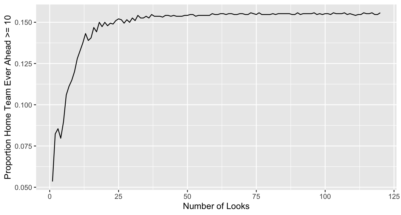
nt   <- 1 : 120
prop <- numeric(120)

g <- function(time, diff) {
  # Look up score differences at specific times
  diffs <- approx(time, diff, xout=times, method='constant', rule=2)$y
  1 * any(diffs >= 10)
}
schedule <- list(30, c(20, 40), c(15, 30, 45))
if(file.exists('prop.rds')) prop <- readRDS('prop.rds') else {
  for(i in 1 : 120) {
    times <- if(i < 4) schedule[[i]] else seq(1, 59, length=i)
    b <- a[, .(any10=g(time, home - away)), by=id]
    prop[i] <- mean(b$any10)
  }
  saveRDS(prop, 'prop.rds')
}

ggplot(mapping=aes(x=nt, y=prop)) + geom_line() +
  xlab('Number of Looks') +
  ylab('Proportion Home Team Ever Ahead >= 10')

The $y$-axis is $\frac{m}{n}$ where $n$ is the number of games in which the home team lost or was tied, and $m$ is the number of such games for which the home team was ever ahead by $\geq 10$ points at any of the equally spaced looks whose number is indicated on the $x$-axis. For one look, consider the halftime score. For two looks, consider scores at minutes 20 and 40. Time three looks at 15, 30, 45. Otherwise looks are equally spaced between minutes 1 and 59.

From the plot, we see that with many data looks there is more than a 0.15 chance of making a false prediction. It is tempting to say that there is a 0.15 chance of being wrong about our team winning, but that’s not what $\alpha$ means. It merely means that we are somewhat likely to trigger our decision if our team doesn’t win. The more we look at the data, the more likely we are to see that a team which eventually/ultimately loses had at least a 10 point lead at some point in the game. The more looks, the more opportunity for a false prediction. The graph is a picture of $\alpha$ versus the number of looks and it gets inflated with more looks. Thus, when making decisions based on the observed data, it is important to know how many times you have observed extreme data, for frequentist decision-making.

Forward Probabilities Have No Multiplicities

Now let’s change our decision rule to be based on a predictive mode, forward looking probability statement about the outcome of interest - whether the home team will win. The observed data is used in calculating the probability, but it is not the direct determinant of our decision rule. Our decision rule is

If the probability (using the NFL’s model) of ultimately winning exceeds 0.90 at any time during the first 55 minutes of a 60 minute game, then we will predict that the home team wins and we can turn off the TV or leave the stadium.

Consider games in which the home team ever had a probability of at least 0.9 of winning with at least 5 minutes remaining.

Code

w <- d
w[, any9 := any(home_prob >= 0.9 & timeleft >= 300), by=id]
w <- w[any9 == TRUE]

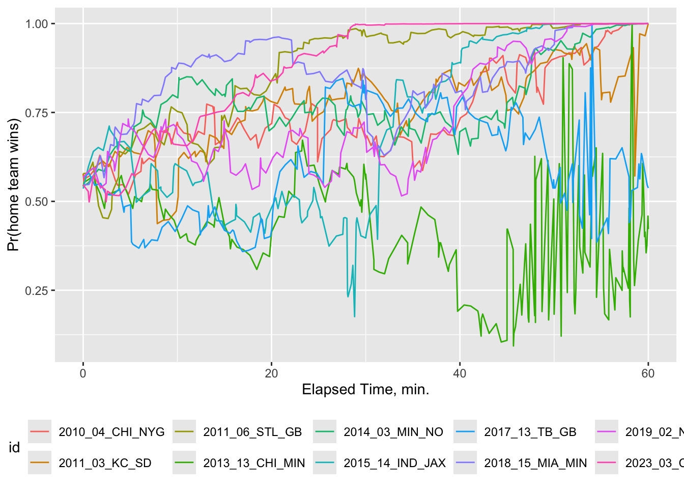
There are 1985 qualifying games. Here is a random sample of 10 of them to show how the winning probability evolved over the course of those games. The NFL model’s predicted probabilities are similar to Bayesian posterior probabilities of treatment effects.

Code

set.seed(2)
ids <- sample(unique(w$id), 10)
ggplot(w[id %in% ids], aes(x=time, y=home_prob, col=id)) +
  geom_line() + xlab('Elapsed Time, min.') + ylab('Pr(home team wins)') +
  theme(legend.position='bottom')

Evolution of win probabilities for ten randomly chosen NFL games in which the home team ever had a probability of winning $\geq 0.9$ with more than 5 minutes remaining

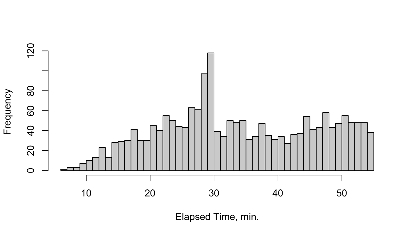
What happens with that decision rule when the data are analyzed after every play? Here is the distribution of times at which the decision rule was triggered (i.e., we decided to stop watching the game) and of the win probabilities at the moment of stopping.

Code

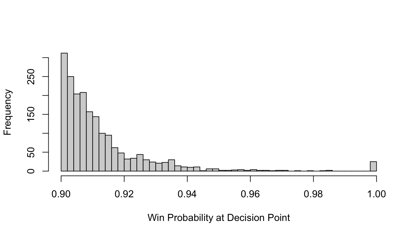
g <- function(time, home_prob) {
  timedec <- min(time[home_prob >= 0.9])
  probdec <- home_prob[time == timedec & home_prob >=0.9][1]
  list(timedec = timedec, probdec=probdec)
}
z <- w[, g(time, home_prob), by=.(id, final_home, final_away)]
with(z, {
  hist(timedec, nclass=50, main='',
        xlab='Elapsed Time, min.')
  hist(probdec, nclass=50, main='',
        xlab='Win Probability at Decision Point')
})

Distribution of times at which we stopped watching the game, i.e., time at first crossing of 0.9 probability

Distribution of win probability at moment we stopped watching

About $\frac{9}{10}$ of the time we get the right answers with continuous data looks—the team that we predicted to win with this decision rule actually won. In fact, the mean predicted probability of winning at the time of stopping is precisely what the observed probability of winning is for the 1985 games analyzed!!

It is worth noting that we could have had a decision rule based on a probability of 0.80 for deciding to stop watching the game. In that case, at the point of deciding to stop watching the game, just over $\frac{4}{5}$ of the time we would have been right, and the mean predicted probability of ultimately winning at the time of stopping would track the observed proportion of times that the home team actually won.

Code

z[, homewon := final_home > final_away]
mn <- function(x) round(mean(x, na.rm=TRUE), 3)
cat('Mean probability at decision point:', z[, mn(probdec)], '\n',
    'Proportion of games in which home team won:', z[, mn(homewon)], '\n', sep='')

Mean probability at decision point:0.913
Proportion of games in which home team won:0.913

So, look all you want … as long as you base your decision rule on the probability of the thing you are interested in - in this case predicting who wins.

Summary

In watching football, sequential looks are made and the decision was to stop watching when the probability of ultimate victory exceeded 0.9. In a clinical trial with sequential looks, one might decide to stop with a conclusion of treatment effectiveness when the probability that the treatment improves outcomes exceeds 0.95.

The accuracy of the win probability is unaffected by the fact that it was used to decide to stop watching the game, just as the accuracy of Bayesian posterior probabilities of efficacy, computed as often as desired as a study unfolds, keep their meaning and accuracy. Contrast this with the backwards time-order probabilities, with probabilities increasing with the number of opportunities for data to be extreme, just as with $\alpha$ in frequentist statistical inference. The fact that Bayesian methods do not attempt to compute probabilities of extreme data, instead dealing only with the probability of “winning”, i.e., the treatment works, makes all the difference in the world. The Bayesian approach is predictive, uses observables, and is about quantifying uncertainty about unknown things. Frequentist hypothesis testing is about quantifying strangeness of data assuming an unobservable unknown thing—the treatment effect is zero. Would you rather know the probability of a positive result when there is nothing, or the probability that a positive result turns out to be nothing? Bayes is about the latter. The frequentist approach insofar as type I assertion probability $\alpha$ is concerned is akin to watching a football game backwards. Bayes is akin to watching the game in the normal fashion, and being interested in the uncertainty about your team winning at any point in the game. Forward thinking eliminates multiplicities while inviting updates to current data.

Reuse

CC BY 4.0

--- title: "Football Multiplicities" author: - name: Frank Harrell url: https://hbiostat.org affiliation: Department of Biostatistics<br>Vanderbilt University School of Medicine - name: Stephen Ruberg url: https://analytixthinking.blog affiliation: Analytix Thinking LLC date: 2024-03-10 date-modified: last-modified categories: [bayes, design, sequential, RCT, accuracy-score, backward-probability, decision-making, forward-probability, inference, multiplicity, prediction, probability, 2024] description: "Traditionally trained statisticians have much difficulty in accepting the absence of multiplicity issues with Bayesian sequential designs, i.e., that Bayesian posterior probabilities do not change interpretation or become miscalibrated just because a stopping rule is in effect. Most statisticians are used to dealing with backwards-information-flow probabilities which do have multiplicity issues, because they must deal with opportunities for data to be extreme. This leads them to believe that Bayesian methods must have some kind of hidden multiplicity problem. The chasm between forward and backwards probabilities is explored with a simple example involving continuous data looks where the ultimate truth is known. The stopping rule is the home NFL team having ≥ 0.9 probability of ultimately winning the game, and the correctness of the Bayesian-style forecast is readily checked." --- ## Background Consider the problem of comparing two treatments by doing squential analyses by avoiding putting too much faith into a fixed sample size design. As shown [here](https://hbiostat.org/bayes/bet/design) the lowest expected sample size will result from looking at the developing data as often as possible in a Bayesian design. The Bayesian approach computes probabilities about unknowns, e.g., the treatment effect, and one can update the current evidence base as often as desired, knowing that the current information has made previous evidence simply obsolete. A stopping rule based on, say a posterior probability of efficacy exceeding 0.95, will result in perfectly calibrated posterior probabilities at the moment of stopping, as demonstrated in a [simple simulation](https://fharrell.com/post/bayes-seq). On the other hand, sequential frequentist analysis gives data more opportunities to be extreme under the null hypothesis, leading to multiplicity challenges if one wants to preserve the type I assertion probability $\alpha$. The real multiplicity issues in the frequentist approach makes traditionally-trained statisticians hesitant to admit that probabilities about parameters are fundamentally different from probabilities about data, and do not involve multiplicities in the sequential testing setting. The purpose of this article is to demonstrate the vast difference between forwards and backwards probabilities in a simple setting in which the ultimate truth is known. ## Data For many years, the U.S. National Football League (NFL) has provided play-by-play updates to carefully constructed probability estimates. The NFL model is for the probability that the home team will ultimately win the game. The model is based on a large number of variables, and sensibly gives heavy weight to the current score and the time left in the 60-minute American football game. The play-by-play NFL data analyzed in this article comes from the [`nflreadr` R package](https://nflreadr.nflverse.com) for the 2008-2023 football seasons^[Ho T, Carl S (2024). `nflreadr`: Download `nflverse` Data. R package version 1.4.0, https://github.com/nflverse/nflreadr, https://nflreadr.nflverse.com]. ```{r} require(Hmisc) require(data.table) require(ggplot2) options(prType='html', datatable.print.topn=50) if(file.exists('nfl.rds')) d <- readRDS('nfl.rds') else { require(nflreadr) d <- load_pbp(2008:2023) d <- as.data.table(d) w <- d[, .(game_id, game_date, game_seconds_remaining, home_score, away_score, total_home_score, total_away_score, home_wp)] w <- upData(w, rename=.q(game_id=id, game_date=date, game_seconds_remaining=timeleft, home_score=final_home, away_score=final_away, total_home_score=home, total_away_score=away, home_wp=home_prob), time=(3600 - timeleft) / 60, date=as.Date(date), units=c(timeleft='seconds', time='minutes'), labels=c(time='Elapsed Time', final_home='Final Score for Home Team', final_away='Final Score for Away Team', home='Home Team Current Score', away='Away Team Current Score', home_prob='Probability Home Team Wins') ) d <- w[! is.na(timeleft)] saveRDS(w, 'nfl.rds', compress='xz') } ``` There are `r length(unique(d$id))` games in the dataset having a total of `r nrow(d)` plays. ## Backwards Probabilities Have Multiplicities Suppose that we want to create a decision rule in the spirit of classical statistics. The decision is about whether our team is going to win the game, so we can safely stop watching the game at a certain point. Classical frequentist statistics emphasizes decision rules that limit what is loosely called the "false positive probability"^["Loosely" because it's not the probability that a positive finding is wrong (i.e., false) but is instead the probability of rejecting a true null hypothesis (i.e., a so-called type I "error"). It's the probability of asserting an effect when no assertion should be made. This conditonal (knows $H_0$ is true) probability is only a distant relative of the probability that an assertion is false, which is an unconditional probability (does not know that $H_0$ is true).] $\alpha$. Classical statistical decision rules are designed around limiting the chance that misleading results _might_ arise, and are not built around merely interpreting the final data. In that spirit, consider all the games in which the home team lost or was tied. ```{r} a <- d[final_home <= final_away] ``` The number of games analyzed is `r length(unique(a$id))`. Let’s consider a decision rule that states * If the home team is ahead at any point in the game by 10 or more points, we will predict that they will win. Perhaps our decision rule would trigger a bet, or we may decide to stop watching the game and do other things. We could execute our decision rule at the end of each quarter of play, or every 5 minutes of game time, or even every time a team scores. Thus, there are many options to define the frequency with which we look at the score and each time there is an opportunity to invoke our decision rule. In theory, one could execute the decision rule after **every** play, but of course the score does not change with every play, so examining our decision rule at this granular level is unnecessary, but it can be instructive for the points we are trying to make. It is obvious that score fluctuations increase with the number of looks, and our decision rule will be triggered more often were the data to be analyzed more often. The probability that the home team in these lost or tied games was ever ahead by $\geq 10$ points is analogous to $\alpha$ in a frequentist testing procedure. The home team's current score margin comprises the data. We are using extreme values of the data to create a decision rule, namely if the home team is ahead by 10 points or more (extreme data), then we predict the home team will win. But we are looking at all the games in which the home team tied or lost. So, we want to know how often our decision rule results in a false positive prediction/decision (or you might say type I "error")^[It's not an "error" but is instead is the probability of making a positive decision when any positive decision is wrong.]. Now, since the score fluctuates during a game, if we take more looks at the data (i.e., the score and specifically if the home team is ahead by 10 points or more), there are multiple opportunities for this to happen throughout a 60 minute game. Let's make the looks equally spaced between the first and fifty-ninth minute of the game, and vary the number of looks from 1 to 120. Capture whether the home team was $\geq 10$ points ahead at each look. ```{r} #| label: lookback #| fig-cap: "The $y$-axis is $\\frac{m}{n}$ where $n$ is the number of games in which the home team lost or was tied, and $m$ is the number of such games for which the home team was ever ahead by $\\geq 10$ points at any of the equally spaced looks whose number is indicated on the $x$-axis. For one look, consider the halftime score. For two looks, consider scores at minutes 20 and 40. Time three looks at 15, 30, 45. Otherwise looks are equally spaced between minutes 1 and 59." #| fig-height: 3.75 nt <- 1 : 120 prop <- numeric(120) g <- function(time, diff) { # Look up score differences at specific times diffs <- approx(time, diff, xout=times, method='constant', rule=2)$y 1 * any(diffs >= 10) } schedule <- list(30, c(20, 40), c(15, 30, 45)) if(file.exists('prop.rds')) prop <- readRDS('prop.rds') else { for(i in 1 : 120) { times <- if(i < 4) schedule[[i]] else seq(1, 59, length=i) b <- a[, .(any10=g(time, home - away)), by=id] prop[i] <- mean(b$any10) } saveRDS(prop, 'prop.rds') } ggplot(mapping=aes(x=nt, y=prop)) + geom_line() + xlab('Number of Looks') + ylab('Proportion Home Team Ever Ahead >= 10') ``` From the plot, we see that with many data looks there is more than a 0.15 chance of making a false prediction. It is tempting to say that there is a 0.15 chance of being wrong about our team winning, but that's not what $\alpha$ means. It merely means that we are somewhat likely to trigger our decision **if** our team doesn't win. The more we look at the data, the more likely we are to see that a team which eventually/ultimately loses had at least a 10 point lead at some point in the game. The more looks, the more opportunity for a false prediction. The graph is a picture of $\alpha$ versus the number of looks and it gets inflated with more looks. Thus, when making decisions based on the observed data, it is important to know how many times you have observed extreme data, for **frequentist** decision-making. ## Forward Probabilities Have No Multiplicities Now let's change our decision rule to be based on a predictive mode, forward looking probability statement about the outcome of interest - whether the home team will win. The observed data is used in calculating the probability, but it is not the direct determinant of our decision rule. Our decision rule is * If the probability (using the NFL's model) of ultimately winning exceeds 0.90 at any time during the first 55 minutes of a 60 minute game, then we will predict that the home team wins and we can turn off the TV or leave the stadium. Consider games in which the home team ever had a probability of at least 0.9 of winning with at least 5 minutes remaining. ```{r} w <- d w[, any9 := any(home_prob >= 0.9 & timeleft >= 300), by=id] w <- w[any9 == TRUE] ``` There are `r length(unique(w$id))` qualifying games. Here is a random sample of 10 of them to show how the winning probability evolved over the course of those games. The NFL model's predicted probabilities are similar to Bayesian posterior probabilities of treatment effects. ```{r} #| label: sample #| fig-cap: "Evolution of win probabilities for ten randomly chosen NFL games in which the home team ever had a probability of winning $\\geq 0.9$ with more than 5 minutes remaining" set.seed(2) ids <- sample(unique(w$id), 10) ggplot(w[id %in% ids], aes(x=time, y=home_prob, col=id)) + geom_line() + xlab('Elapsed Time, min.') + ylab('Pr(home team wins)') + theme(legend.position='bottom') ``` What happens with that decision rule when the data are analyzed after every play? Here is the distribution of times at which the decision rule was triggered (i.e., we decided to stop watching the game) and of the win probabilities at the moment of stopping. ```{r} #| label: hist #| layout-nrow: 2 #| fig-height: 4 #| fig-subcap: #| - "Distribution of times at which we stopped watching the game, i.e., time at first crossing of 0.9 probability" #| - "Distribution of win probability at moment we stopped watching" g <- function(time, home_prob) { timedec <- min(time[home_prob >= 0.9]) probdec <- home_prob[time == timedec & home_prob >=0.9][1] list(timedec = timedec, probdec=probdec) } z <- w[, g(time, home_prob), by=.(id, final_home, final_away)] with(z, { hist(timedec, nclass=50, main='', xlab='Elapsed Time, min.') hist(probdec, nclass=50, main='', xlab='Win Probability at Decision Point') }) ``` About $\frac{9}{10}$ of the time we get the right answers with continuous data looks---the team that we predicted to win with this decision rule actually won. In fact, the mean predicted probability of winning at the time of stopping is precisely what the observed probability of winning is for the 1985 games analyzed!! [It is worth noting that we could have had a decision rule based on a probability of 0.80 for deciding to stop watching the game. In that case, at the point of deciding to stop watching the game, just over $\frac{4}{5}$ of the time we would have been right, and the mean predicted probability of ultimately winning at the time of stopping would track the observed proportion of times that the home team actually won.]{.aside} ```{r} z[, homewon := final_home > final_away] mn <- function(x) round(mean(x, na.rm=TRUE), 3) cat('Mean probability at decision point:', z[, mn(probdec)], '\n', 'Proportion of games in which home team won:', z[, mn(homewon)], '\n', sep='') ``` So, look all you want ... as long as you base your decision rule on the probability of the thing you are interested in - in this case predicting who wins. ## Summary In watching football, sequential looks are made and the decision was to stop watching when the probability of ultimate victory exceeded 0.9. In a clinical trial with sequential looks, one might decide to stop with a conclusion of treatment effectiveness when the probability that the treatment improves outcomes exceeds 0.95. The accuracy of the win probability is unaffected by the fact that it was used to decide to stop watching the game, just as the accuracy of Bayesian posterior probabilities of efficacy, computed as often as desired as a study unfolds, keep their meaning and accuracy. Contrast this with the backwards time-order probabilities, with probabilities increasing with the number of opportunities for data to be extreme, just as with $\alpha$ in frequentist statistical inference. The fact that Bayesian methods do not attempt to compute probabilities of extreme data, instead dealing only with the probability of "winning", i.e., the treatment works, makes all the difference in the world. The Bayesian approach is predictive, uses observables, and is about quantifying uncertainty about unknown things. Frequentist hypothesis testing is about quantifying strangeness of data **assuming** an unobservable unknown thing---the treatment effect is zero. Would you rather know the [probability of a positive result **when** there is nothing, or the probability that a positive result **turns out to be** nothing](https://hbiostat.org/bbr/alpha)? Bayes is about the latter. The frequentist approach insofar as type I assertion probability $\alpha$ is concerned is akin to watching a football game backwards. Bayes is akin to watching the game in the normal fashion, and being interested in the uncertainty about your team winning at any point in the game. Forward thinking eliminates multiplicities while inviting updates to current data.