How Does a Compound Symmetric Correlation Structure Translate to a Markov Model?
Random intercepts in a model induce a compound symmetric correlation structure in which the correlation between two responses on the same subject have the same correlation no matter the time gap between the responses. How does one capture such an unnatural structure using a Markov semiparametric model?
Let’s generate some data with repeatedly measured outcome per subject where the outcome is a coursened continuous response from a linear model, treated as ordinal, and the random effects have a \(N(0, 0.25^2)\) distribution. Generate 5000 subjects having 10 measurements each.
Code
n <- 5000   # subjects
set.seed(2)
re <- rnorm(n) * 0.25
X  <- runif(n)   # baseline covariate, will be duplicated over time within subject
m  <- 10         # measurements per subject

id <- rep(1 : n, each = m)
x  <- X[id]
y  <- x + re[id] + rnorm(n * m) * 0.5
y  <- pmin(2, pmax(-1, y))   # curtail y
y  <- round(4 * y)           # coursen it
d  <- data.table(id, x, y)
d[, t := 1 : .N, by=id]
# Make short and wide dataset
w <- dcast(d[, .(id, t, y)],
           id ~ t, value.var='y')
r <- cor(as.matrix(w[, -1]), use='pairwise.complete.obs',
         method='pearson')
p <- plotCorrM(r)
p[[1]]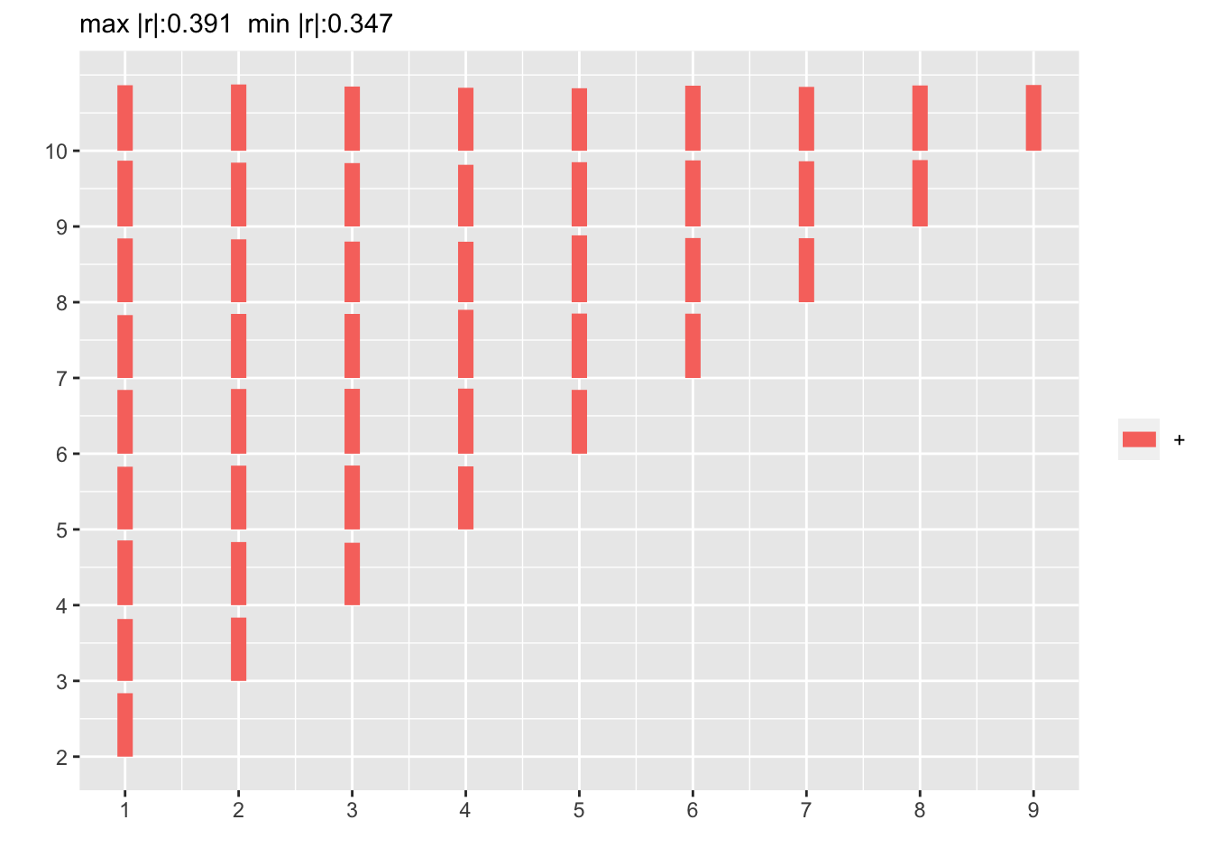
Code
p[[2]] + ylim(0,1)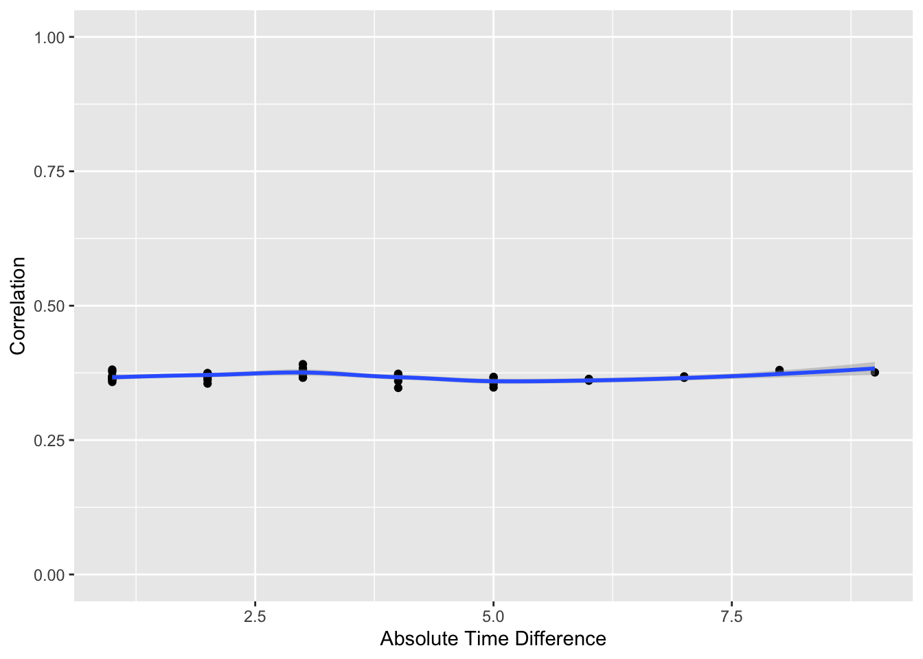
The flat correlation pattern vs. time gap is as expected.
Fit a first-order Markov PO model to times 2, 3, …, 10. Allow previous y to interact with a flexible function of time.
Code
d[, yprev := shift(y), by=id]
f <- orm(y ~ pol(x, 2) + pol(yprev, 2) * pol(t, 3), data=d)
anova(f)
Wald Statistics for y |
|||
| χ2 | d.f. | P | |
|---|---|---|---|
| x | 5565.78 | 2 | <0.0001 |
| Nonlinear | 6.28 | 1 | 0.0122 |
| yprev (Factor+Higher Order Factors) | 1696.29 | 8 | <0.0001 |
| All Interactions | 3.77 | 6 | 0.7082 |
| Nonlinear (Factor+Higher Order Factors) | 0.68 | 4 | 0.9544 |
| t (Factor+Higher Order Factors) | 5.94 | 9 | 0.7458 |
| All Interactions | 3.77 | 6 | 0.7082 |
| Nonlinear (Factor+Higher Order Factors) | 2.01 | 6 | 0.9188 |
| yprev × t (Factor+Higher Order Factors) | 3.77 | 6 | 0.7082 |
| Nonlinear | 1.50 | 5 | 0.9126 |
| Nonlinear Interaction : f(A,B) vs. AB | 1.50 | 5 | 0.9126 |
| f(A,B) vs. Af(B) + Bg(A) | 0.31 | 2 | 0.8560 |
| Nonlinear Interaction in yprev vs. Af(B) | 0.43 | 3 | 0.9346 |
| Nonlinear Interaction in t vs. Bg(A) | 1.38 | 4 | 0.8472 |
| TOTAL NONLINEAR | 8.41 | 9 | 0.4938 |
| TOTAL NONLINEAR + INTERACTION | 10.65 | 10 | 0.3853 |
| TOTAL | 11187.92 | 13 | <0.0001 |
Code
g <- orm(y ~ pol(x,2) + yprev + t, data=d)
g
Logistic (Proportional Odds) Ordinal Regression Model
orm(formula = y ~ pol(x, 2) + yprev + t, data = d)
Frequencies of Responses
  -4   -3   -2   -1    0    1    2    3    4    5    6    7    8
 634 1012 2109 3494 5106 6413 6908 6529 5315 3620 2106 1090  664
Frequencies of Missing Values Due to Each Variable
    y     x yprev     t
    0     0  5000     0
| Model Likelihood Ratio Test |
Discrimination Indexes |
Rank Discrim. Indexes |
|
|---|---|---|---|
| Obs 45000 | LR χ2 12078.42 | R2 0.238 | ρ 0.488 |
| Distinct Y 13 | d.f. 4 | R24,45000 0.235 | |
| Y0.5 2 | Pr(>χ2) <0.0001 | R24,44374.5 0.238 | |
| max |∂log L/∂β| 1×10⁻⁶ | Score χ2 12153.40 | |Pr(Y ≥ median)-½| 0.194 | |
| Pr(>χ2) <0.0001 |
| β | S.E. | Wald Z | Pr(>|Z|) | |
|---|---|---|---|---|
| x | 2.7847 | 0.1160 | 24.01 | <0.0001 |
| x2 | -0.2728 | 0.1113 | -2.45 | 0.0142 |
| yprev | 0.1551 | 0.0038 | 41.14 | <0.0001 |
| t | 0.0040 | 0.0032 | 1.24 | 0.2136 |
There was no evidence for a nonlinear effect of previous y, or an interaction between previous value and time.
Fifth-Order Markov Model with Linear Effects
Code
d[, yprev2 := shift(yprev),  by=id]
d[, yprev3 := shift(yprev2), by=id]
d[, yprev4 := shift(yprev3), by=id]
d[, yprev5 := shift(yprev4), by=id]
f <- orm(y ~ pol(x, 2) + yprev + yprev2 + yprev3 + yprev4 + yprev5 + t, data=d)
f
Logistic (Proportional Odds) Ordinal Regression Model
orm(formula = y ~ pol(x, 2) + yprev + yprev2 + yprev3 + yprev4 +
    yprev5 + t, data = d)
Frequencies of Responses
  -4   -3   -2   -1    0    1    2    3    4    5    6    7    8
 337  540 1183 1958 2754 3601 3855 3647 2964 2015 1167  622  357

| Model Likelihood Ratio Test |
Discrimination Indexes |
Rank Discrim. Indexes |
|
|---|---|---|---|
| Obs 25000 | LR χ2 8641.08 | R2 0.295 | ρ 0.538 |
| Distinct Y 13 | d.f. 8 | R28,25000 0.292 | |
| Y0.5 2 | Pr(>χ2) <0.0001 | R28,24649.9 0.295 | |
| max |∂log L/∂β| 2×10⁻⁶ | Score χ2 8831.52 | |Pr(Y ≥ median)-½| 0.212 | |
| Pr(>χ2) <0.0001 |
| β | S.E. | Wald Z | Pr(>|Z|) | |
|---|---|---|---|---|
| x | 1.6573 | 0.1579 | 10.49 | <0.0001 |
| x2 | -0.2336 | 0.1494 | -1.56 | 0.1180 |
| yprev | 0.0949 | 0.0053 | 17.91 | <0.0001 |
| yprev2 | 0.0956 | 0.0053 | 18.12 | <0.0001 |
| yprev3 | 0.1062 | 0.0053 | 20.07 | <0.0001 |
| yprev4 | 0.0882 | 0.0052 | 16.80 | <0.0001 |
| yprev5 | 0.0771 | 0.0052 | 14.70 | <0.0001 |
| t | 0.0060 | 0.0079 | 0.76 | 0.4488 |
Code
anova(f, yprev2, yprev3, yprev4, yprev5)Wald Statistics for y |
|||
| χ2 | d.f. | P | |
|---|---|---|---|
| yprev2 | 328.18 | 1 | <0.0001 |
| yprev3 | 402.61 | 1 | <0.0001 |
| yprev4 | 282.37 | 1 | <0.0001 |
| yprev5 | 216.13 | 1 | <0.0001 |
| TOTAL | 1833.15 | 4 | <0.0001 |
For the compound symmetric correlation structure the effect of all previous values of y is the same, and all lags are important.
See if the mean of all previous values can replace all the individual lagged variables.
Code
d[, ypmean := (yprev + yprev2 + yprev3 + yprev4 + yprev5) / 5]
fm <- orm(y ~ pol(x, 2) + ypmean + t, data=d)
fm
Logistic (Proportional Odds) Ordinal Regression Model
orm(formula = y ~ pol(x, 2) + ypmean + t, data = d)
Frequencies of Responses
  -4   -3   -2   -1    0    1    2    3    4    5    6    7    8
 337  540 1183 1958 2754 3601 3855 3647 2964 2015 1167  622  357
Frequencies of Missing Values Due to Each Variable
     y      x ypmean      t
     0      0  25000      0
| Model Likelihood Ratio Test |
Discrimination Indexes |
Rank Discrim. Indexes |
|
|---|---|---|---|
| Obs 25000 | LR χ2 8626.32 | R2 0.295 | ρ 0.538 |
| Distinct Y 13 | d.f. 4 | R24,25000 0.292 | |
| Y0.5 2 | Pr(>χ2) <0.0001 | R24,24649.9 0.295 | |
| max |∂log L/∂β| 2×10⁻⁶ | Score χ2 8815.53 | |Pr(Y ≥ median)-½| 0.211 | |
| Pr(>χ2) <0.0001 |
| β | S.E. | Wald Z | Pr(>|Z|) | |
|---|---|---|---|---|
| x | 1.6530 | 0.1579 | 10.47 | <0.0001 |
| x2 | -0.2297 | 0.1494 | -1.54 | 0.1243 |
| ypmean | 0.4618 | 0.0087 | 52.90 | <0.0001 |
| t | 0.0061 | 0.0079 | 0.78 | 0.4355 |
Code
AIC(fm); AIC(f)[1] 107771.7 [1] 107765
The previous model is better but by an inconsequential amount. The compound symmetric correlation pattern is reproduced by conditioning on the mean of all previous response values.
Combined Markov and Random Effects Model
Add random intercepts and see if lags are still important in a Bayesian PO model.
Code
require(rmsb)
options(mc.cores=4, rmsb.backend='cmdstan')  # took 7m on 4 cores (4 chains)
b <- blrm(y ~ pol(x, 2) + yprev + yprev2 + yprev3 + yprev4 + yprev5 + t +
          cluster(id), data=d, file='corstruct-b.rds')
b
Bayesian Proportional Odds Ordinal Logistic Model
Dirichlet Priors With Concentration Parameter 0.187 for Intercepts
blrm(formula = y ~ pol(x, 2) + yprev + yprev2 + yprev3 + yprev4 +
    yprev5 + t + cluster(id), data = d, file = "corstruct-b.rds")
Frequencies of Responses
  -4   -3   -2   -1    0    1    2    3    4    5    6    7    8
 337  540 1183 1958 2754 3601 3855 3647 2964 2015 1167  622  357

| Mixed Calibration/ Discrimination Indexes |
Discrimination Indexes |
Rank Discrim. Indexes |
|
|---|---|---|---|
| Obs 25000 | B 0.194 [0.194, 0.194] | g 1.301 [1.273, 1.327] | C 0.704 [0.704, 0.704] |
| Draws 4000 | gp 0.263 [0.259, 0.267] | Dxy 0.408 [0.408, 0.409] | |
| Chains 4 | EV 0.217 [0.21, 0.223] | ||
| Time 369.7s | v 1.29 [1.237, 1.342] | ||
| p 8 | vp 0.053 [0.051, 0.054] | ||
Cluster on id |
|||
| Clusters 5000 | |||
| σγ 0.0328 [1e-04, 0.0966] |
| Mean β | Median β | S.E. | Lower | Upper | Pr(β>0) | Symmetry | |
|---|---|---|---|---|---|---|---|
| x | 1.6592 | 1.6587 | 0.1567 | 1.3281 | 1.9378 | 1.0000 | 0.98 |
| x2 | -0.2314 | -0.2334 | 0.1482 | -0.5081 | 0.0684 | 0.0583 | 1.03 |
| yprev | 0.0946 | 0.0946 | 0.0052 | 0.0847 | 0.1052 | 1.0000 | 0.99 |
| yprev2 | 0.0954 | 0.0954 | 0.0051 | 0.0855 | 0.1048 | 1.0000 | 0.95 |
| yprev3 | 0.1061 | 0.1061 | 0.0054 | 0.0955 | 0.1166 | 1.0000 | 1.03 |
| yprev4 | 0.0883 | 0.0882 | 0.0049 | 0.0784 | 0.0977 | 1.0000 | 0.99 |
| yprev5 | 0.0773 | 0.0773 | 0.0052 | 0.0674 | 0.0875 | 1.0000 | 1.01 |
| t | 0.0061 | 0.0061 | 0.0083 | -0.0093 | 0.0228 | 0.7562 | 1.03 |
With the lagged variables in the model the standard deviation \(\sigma_\gamma\) of the random effects is very small, and oddly enough the previous values remain important. I conjecture that if the lagged variables were removed \(\sigma_\gamma\) would be much larger and the model would be about as good.
Computing Environment
`R version 4.3.2 (2023-10-31) Platform: aarch64-apple-darwin20 (64-bit) Running under: macOS Ventura 13.6.1 Matrix products: default BLAS: /Library/Frameworks/R.framework/Versions/4.3-arm64/Resources/lib/libRblas.0.dylib LAPACK: /Library/Frameworks/R.framework/Versions/4.3-arm64/Resources/lib/libRlapack.dylib; LAPACK version 3.11.0 attached base packages: [1] stats graphics grDevices utils datasets methods base other attached packages: [1] rmsb_1.0-0 ggplot2_3.4.4 data.table_1.14.8 rms_6.8-0 [5] Hmisc_5.1-2To cite R in publications use:
R Core Team (2023). R: A Language and Environment for Statistical Computing. R Foundation for Statistical Computing, Vienna, Austria. https://www.R-project.org/.
To cite the Hmisc package in publications use:
Harrell Jr F (2023). Hmisc: Harrell Miscellaneous. R package version 5.1-2, https://hbiostat.org/R/Hmisc/.
To cite the rms package in publications use:
Harrell Jr FE (2023). rms: Regression Modeling Strategies. R package version 6.8-0, https://github.com/harrelfe/rms, https://hbiostat.org/R/rms/.
To cite the rmsb package in publications use:
Harrell F (2023). rmsb: Bayesian Regression Modeling Strategies. R package version 1.0-0, https://hbiostat.org/R/rmsb/.
To cite the data.table package in publications use:
Dowle M, Srinivasan A (2023). data.table: Extension of ‘data.frame’. R package version 1.14.8, https://CRAN.R-project.org/package=data.table.
To cite the ggplot2 package in publications use:
Wickham H (2016). ggplot2: Elegant Graphics for Data Analysis. Springer-Verlag New York. ISBN 978-3-319-24277-4, https://ggplot2.tidyverse.org.
`{=html}