Implications of Interactions in Treatment Comparisons
Transportability of treatment effect estimates depends on the nature of interactions. In the absence of interactions, an effect estimated on a highly selected sample will apply to a much different population. In an observational study, the corresponding condition is that there need be no overlap in the baseline distribution of non-interacting factors. When there is an interaction, one can live with only a small to moderate amount of overlap in characteristics (between randomized vs. population target or between characteristics of treated vs. non-treated patients in an observational study) if the interaction is of a simple form. With more overlap, interactions can be complex (if modeled) and results from analysis of the sample will allow estimation of treatment effect in a different population. In the absence of significant overlap, confidence bands allowing for interaction properly inform the researcher about uncertainties in treatment effects.
Randomized clinical trials do not require representative patients; they require representative treatment effects. Generalizability of randomized trial findings for relative efficacy comes from one of three things:
- true absence of interactions,
- interacting factors have a similar distribution in the RCT as in the target population, or
- the RCT sample has enough representation of the distribution of interacting factors to allow them to be modeled and used to estimate treatment effects in target patients, and the researcher knows to include these interactions in her model.
Note: For shaded boxes marked with ⮩ click on the box to view the associated text.
Background
It is a commonly held belief that clinical trials, to provide treatment effects that are generalizable to a population, must use a sample that reflects that population’s characteristics. The confusion stems from the fact that if one were interested in estimating an average outcome for patients given treatment A, one would need a random sample from the target population. But clinical trials are not designed to estimate absolutes; they are designed to estimate differences as discussed further here. These differences, when measured on a scale for which treatment differences are allowed mathematically to be constant (e.g., difference in means, odds ratios, hazard ratios), show remarkable constancy as judged by a large number of published forest plots. What would make a treatment estimate (relative efficacy) not be transportable to another population? A requirement for non-generalizability is the existence of interactions with treatment such that the interacting factors have a distribution in the sample that is much different from the distribution in the population.
A related problem is the issue of overlap in observational studies. Researchers are taught that non-overlap makes observational treatment comparisons impossible. This is only true when the characteristic whose distributions don’t overlap between treatment groups interacts with treatment. The purpose of this article is to explore interactions in these contexts.
As a side note, if there is an interaction between treatment and a covariate, standard propensity score analysis will completely miss it.
For the following I assume that there is at most one variable (patient age) interacting with treatment effect. The data generating and analysis models are logistic models containing only age and treatment. I also assume that the goal is to assess efficacy isolated from net clinical benefit, e.g., we are not taking side effects into account.
Situations addressed below come from the following 2 × 2 × 2 × 3 combinations:
- randomized vs. observational study
- true data generating process has no interaction with age vs. has a linear interaction
- overlap in ages between RCT sample and target population (or between treatments in an observational study) is completely absent vs. partial overlap in the age distribution
- fitted model is linear with no interaction, has a linear interaction, or has a spline function of age interacting with treatment
I’ll explore what happens when interaction should be included in a model but is omitted, when an interaction is not needed but is included in the model, and when the interaction is simple but is allowed to be complex.
Generalizability of Randomized Clinical Trials
When the outcome generating process in a randomized clinical trial (RCT) is such that treatment does not interact with any baseline patient characteristic over the range of characteristics seen in the union of the RCT and the population, the estimate of relative efficacy (e.g., odds ratio) of treatment applies to every patient in the population. In addition to computing patient-specific odds ratios (ORs), one can easily compute patient-specific absolute risk reductions from treatment as shown here. If one allows for needless interaction terms, it is possible to get poor extrapolation of treatment benefit in unrepresented patient groups, unless the estimated interaction effects are very small (not guaranteed until the sample size is very large).
True Model Has No Treatment Interactions
Estimation of Treatment Effect in Population With No Overlap
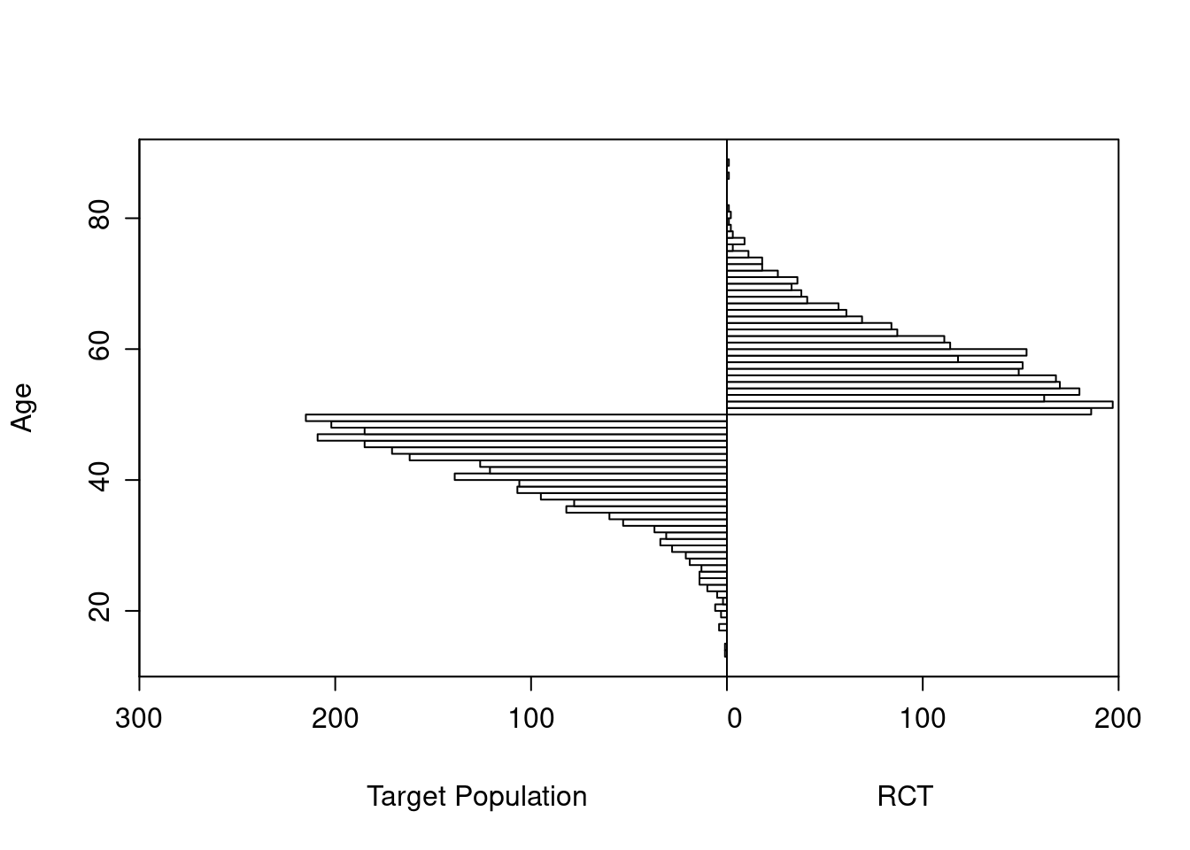
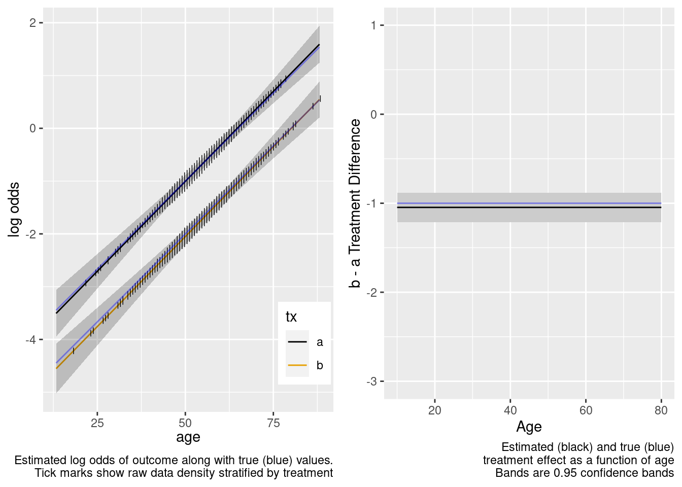
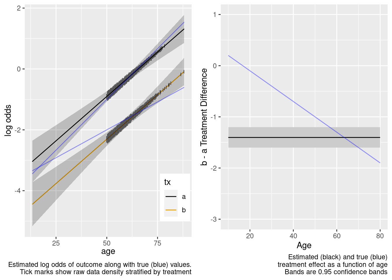
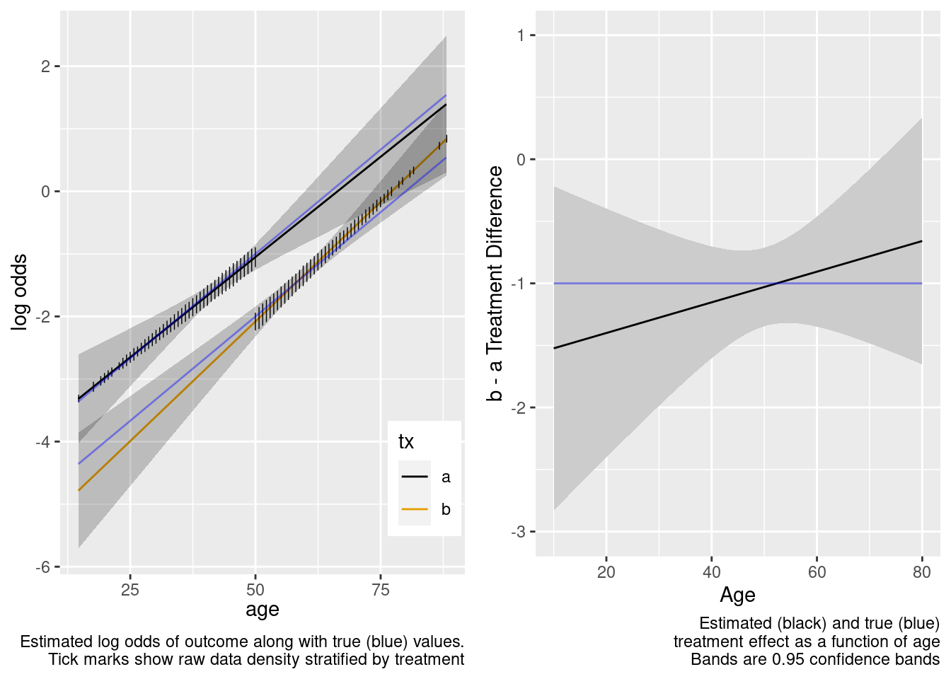
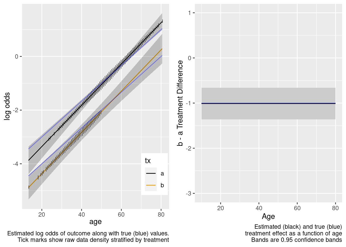
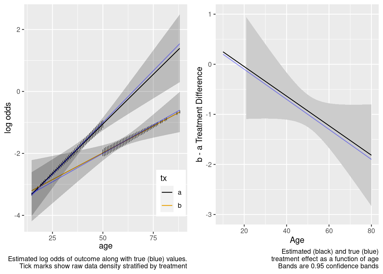
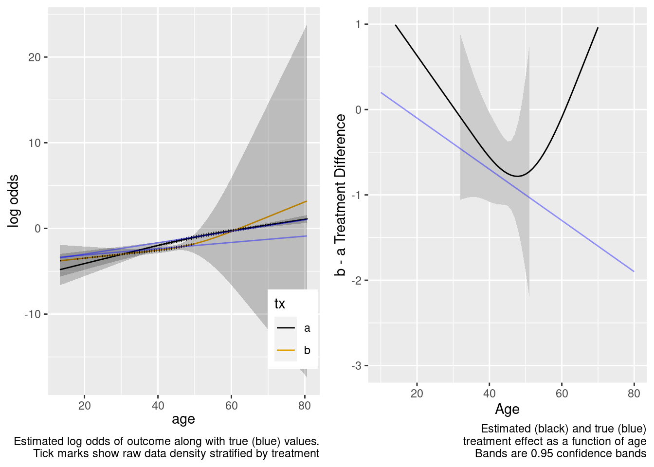
As an example, consider a simulated study of about 2500 patients with a binary outcome where the model contains only age and treatment, the age effect is linear, and there is no interaction. The following R code simulates the data from a hypothetical population, fits a binary logistic model, and displays estimated log odds of outcome vs. age and treatment (left panel) and the estimated age-specific treatment effect (right panel), along with the true population values for both panels over the whole range of age. The RCT excluded those with age < 50 but the target population is exactly those patients. Tick marks on fitted curves display treatment-specific raw data spike histograms.
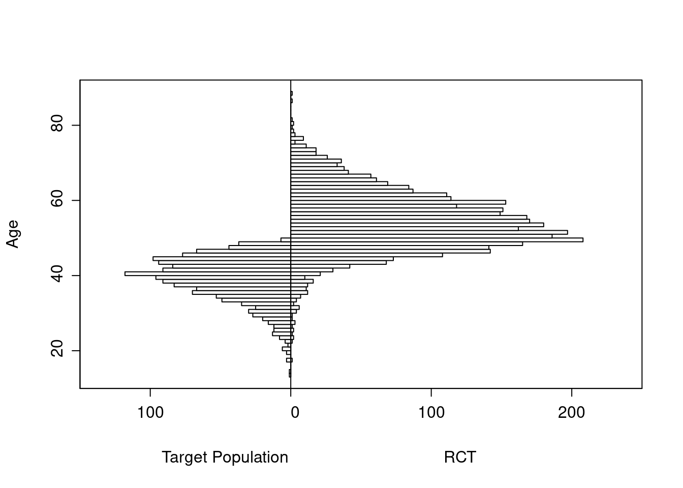
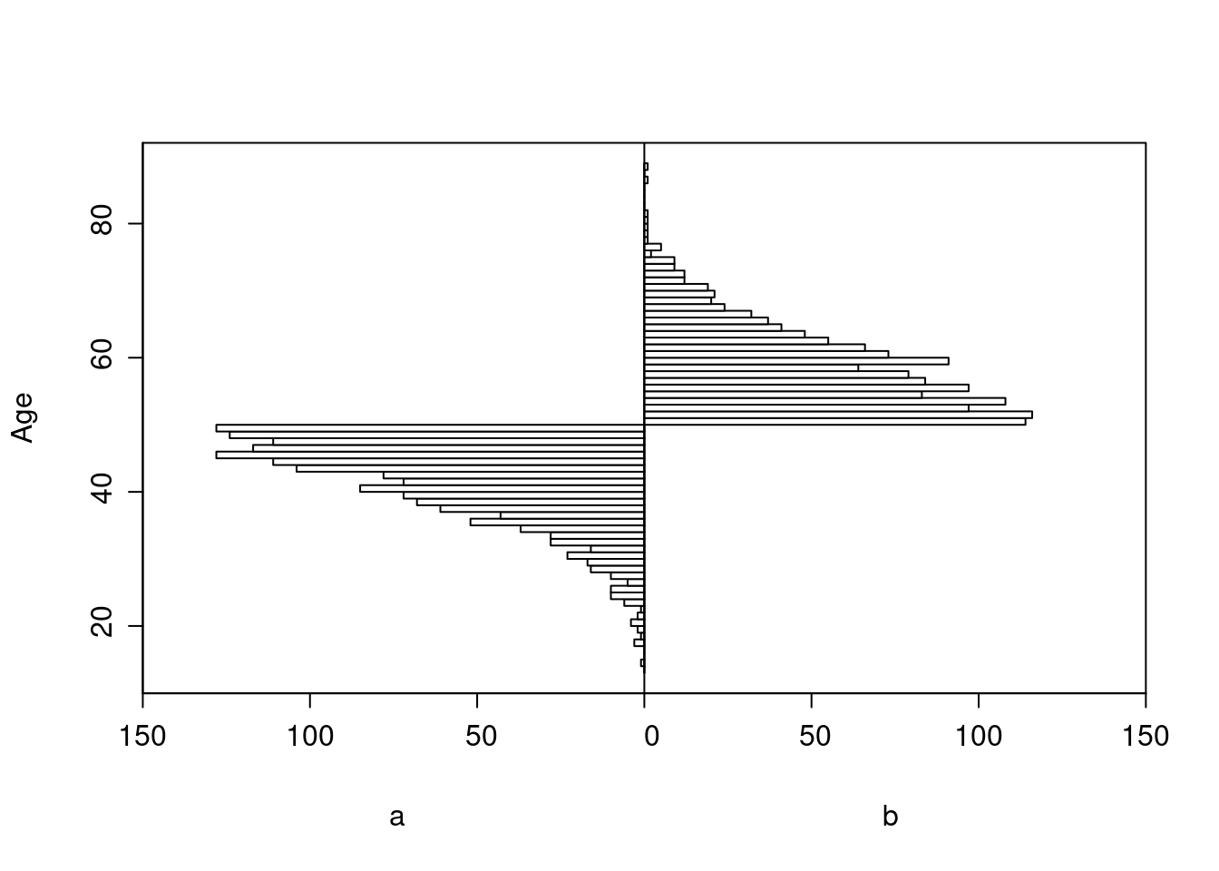
The original age range is 13.3 - 88.1 in 5000 subjects, and the clinical trial includes 2461 of the subjects.
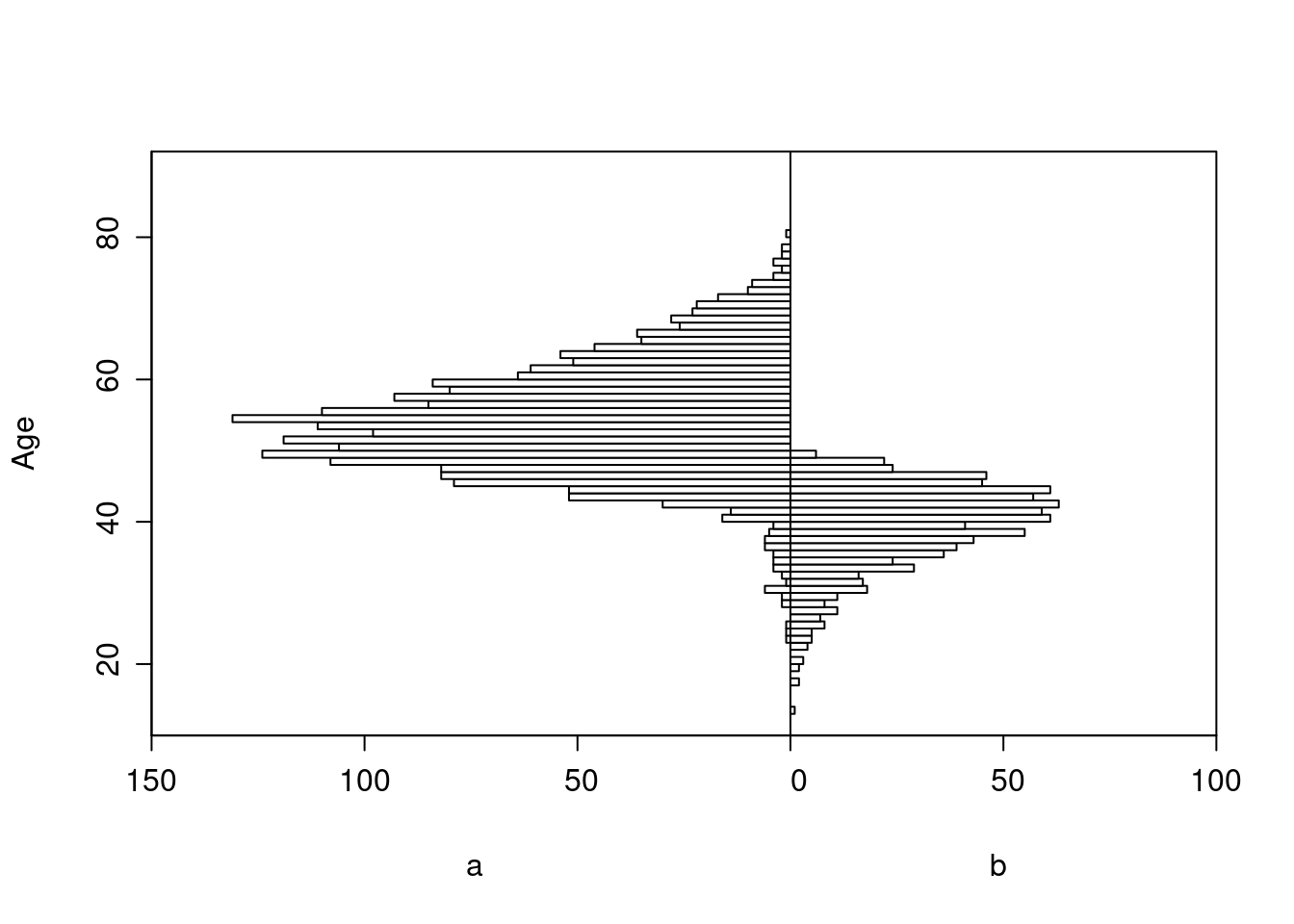
Age distributions in the target population as compared to the RCT sample are shown below.
Logistic Regression Model
lrm(formula = y ~ tx + age, data = d)
Frequencies of Missing Values Due to Each Variable
    y   tx  age
 2539    0    0
|
Model Likelihood Ratio Test |
Discrimination Indexes |
Rank Discrim. Indexes |
|
|---|---|---|---|
| Obs 2461 | LR χ2 211.90 | R2 0.117 | C 0.679 |
| 0 1735 | d.f. 2 | R22,2461 0.082 | Dxy 0.357 |
| 1 726 | Pr(>χ2) <0.0001 | R22,1535.5 0.128 | γ 0.357 |
| max |∂log L/∂β| 2×10⁻⁷ | Brier 0.190 | τa 0.149 |
| β | S.E. | Wald Z | Pr(>|Z|) | |
|---|---|---|---|---|
| Intercept | -4.3508 | 0.4387 | -9.92 | <0.0001 |
| tx=b | -1.0992 | 0.0959 | -11.46 | <0.0001 |
| age | 0.0674 | 0.0074 | 9.05 | <0.0001 |
Wald Statistics for y
|
|||
| χ2 | d.f. | P | |
|---|---|---|---|
| tx | 131.30 | 1 | <0.0001 |
| age | 81.95 | 1 | <0.0001 |
| TOTAL | 189.63 | 2 | <0.0001 |
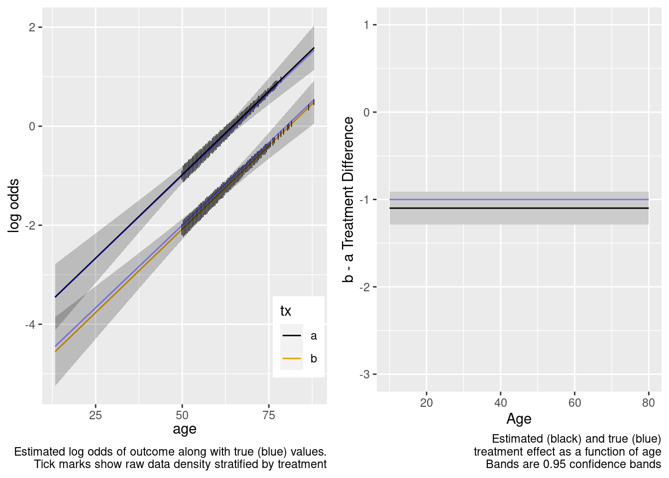
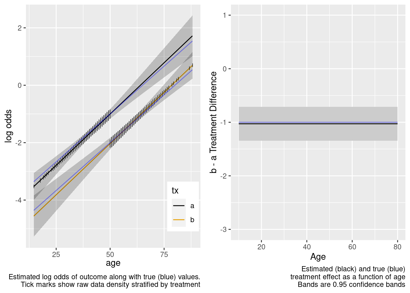
Extrapolation to the younger population is fine even with no younger patients in the RCT. Confidence bands are computed under the assumption of an additive linear age effect.
This is the correct model.
Logistic Regression Model
lrm(formula = y ~ tx * age, data = d)
Frequencies of Missing Values Due to Each Variable
    y   tx  age
 2539    0    0
|
Model Likelihood Ratio Test |
Discrimination Indexes |
Rank Discrim. Indexes |
|
|---|---|---|---|
| Obs 2461 | LR χ2 212.02 | R2 0.117 | C 0.679 |
| 0 1735 | d.f. 3 | R23,2461 0.081 | Dxy 0.357 |
| 1 726 | Pr(>χ2) <0.0001 | R23,1535.5 0.127 | γ 0.357 |
| max |∂log L/∂β| 5×10⁻⁶ | Brier 0.190 | τa 0.149 |
| β | S.E. | Wald Z | Pr(>|Z|) | |
|---|---|---|---|---|
| Intercept | -4.2193 | 0.5852 | -7.21 | <0.0001 |
| tx=b | -1.3998 | 0.8939 | -1.57 | 0.1174 |
| age | 0.0652 | 0.0100 | 6.53 | <0.0001 |
| tx=b × age | 0.0051 | 0.0150 | 0.34 | 0.7351 |
Wald Statistics for y
|
|||
| χ2 | d.f. | P | |
|---|---|---|---|
| tx (Factor+Higher Order Factors) | 131.11 | 2 | <0.0001 |
| All Interactions | 0.11 | 1 | 0.7351 |
| age (Factor+Higher Order Factors) | 82.19 | 2 | <0.0001 |
| All Interactions | 0.11 | 1 | 0.7351 |
| tx × age (Factor+Higher Order Factors) | 0.11 | 1 | 0.7351 |
| TOTAL | 188.87 | 3 | <0.0001 |
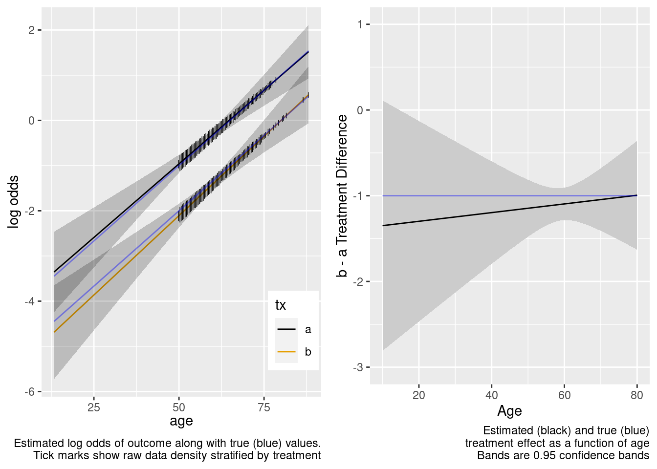
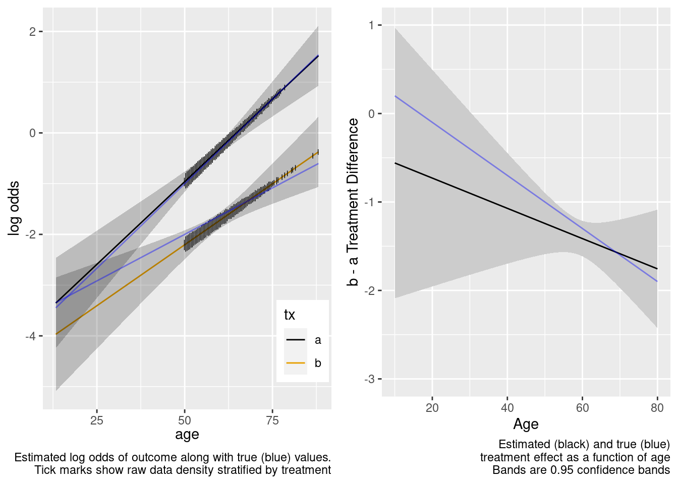
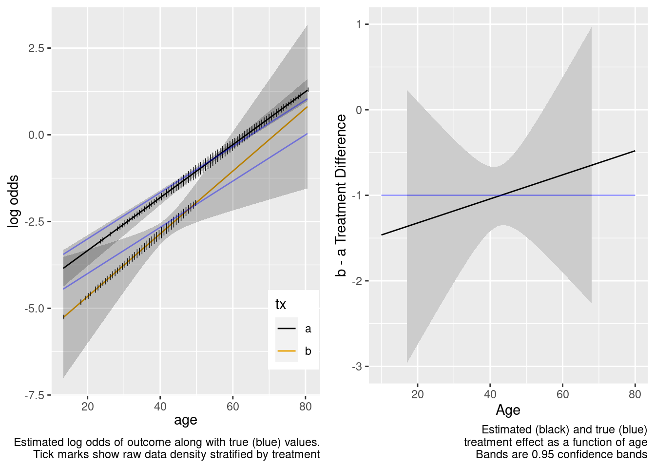
Note that the close-to-zero estimated interaction in the trial sample led to an appropriate extrapolation to the target population of age < 50, with the confidence bands getting wider.
Now see what happens when age is unnecessarily allowed to have a nonlinear non-additive effect, by fitting a model that is quadratic in age interacting with treatment.
This model included an unnecessary linear interaction term.
Logistic Regression Model
lrm(formula = form, data = d, tol = 1e-12)
Frequencies of Missing Values Due to Each Variable
    y   tx  age
 2539    0    0
|
Model Likelihood Ratio Test |
Discrimination Indexes |
Rank Discrim. Indexes |
|
|---|---|---|---|
| Obs 2461 | LR χ2 214.13 | R2 0.119 | C 0.679 |
| 0 1735 | d.f. 7 | R27,2461 0.081 | Dxy 0.358 |
| 1 726 | Pr(>χ2) <0.0001 | R27,1535.5 0.126 | γ 0.358 |
| max |∂log L/∂β| 2×10⁻⁵ | Brier 0.190 | τa 0.149 |
| β | S.E. | Wald Z | Pr(>|Z|) | |
|---|---|---|---|---|
| Intercept | -3.0988 | 1.2779 | -2.42 | 0.0153 |
| tx=b | -1.3609 | 2.0910 | -0.65 | 0.5151 |
| age | 0.0445 | 0.0231 | 1.93 | 0.0542 |
| age’ | 0.2124 | 0.2213 | 0.96 | 0.3372 |
| age’’ | -0.4384 | 0.4906 | -0.89 | 0.3716 |
| tx=b × age | 0.0043 | 0.0376 | 0.11 | 0.9087 |
| tx=b × age’ | 0.0067 | 0.3136 | 0.02 | 0.9829 |
| tx=b × age’’ | -0.0141 | 0.6574 | -0.02 | 0.9829 |
Wald Statistics for y
|
|||
| χ2 | d.f. | P | |
|---|---|---|---|
| tx (Factor+Higher Order Factors) | 131.33 | 4 | <0.0001 |
| All Interactions | 0.11 | 3 | 0.9910 |
| age (Factor+Higher Order Factors) | 85.26 | 6 | <0.0001 |
| All Interactions | 0.11 | 3 | 0.9910 |
| Nonlinear (Factor+Higher Order Factors) | 2.11 | 4 | 0.7151 |
| tx × age (Factor+Higher Order Factors) | 0.11 | 3 | 0.9910 |
| Nonlinear | 0.00 | 2 | 0.9998 |
| Nonlinear Interaction : f(A,B) vs. AB | 0.00 | 2 | 0.9998 |
| TOTAL NONLINEAR | 2.11 | 4 | 0.7151 |
| TOTAL NONLINEAR + INTERACTION | 2.23 | 5 | 0.8162 |
| TOTAL | 190.78 | 7 | <0.0001 |
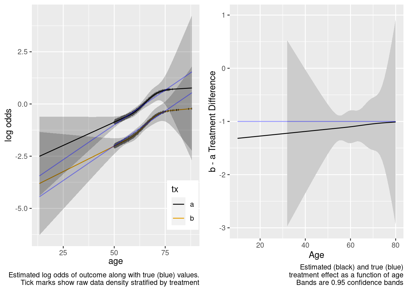
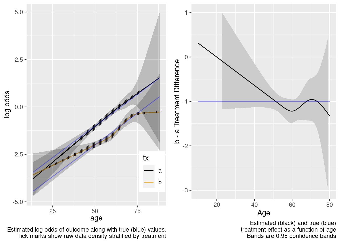
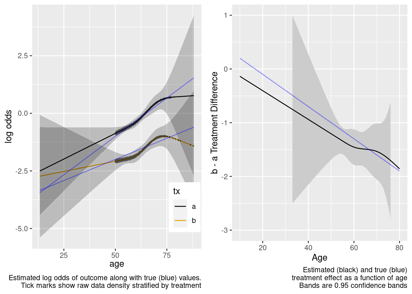
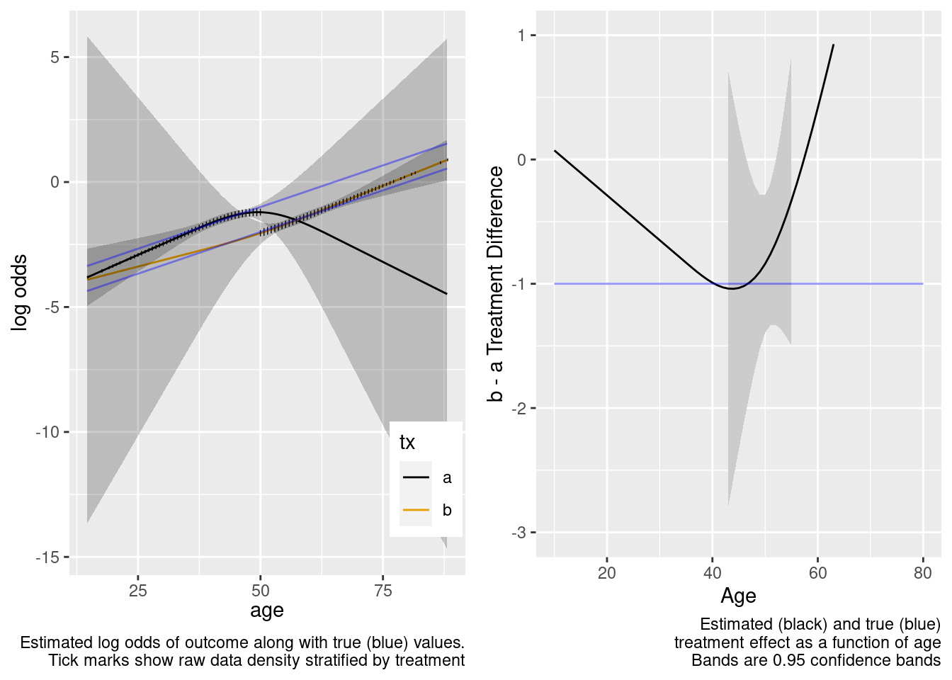
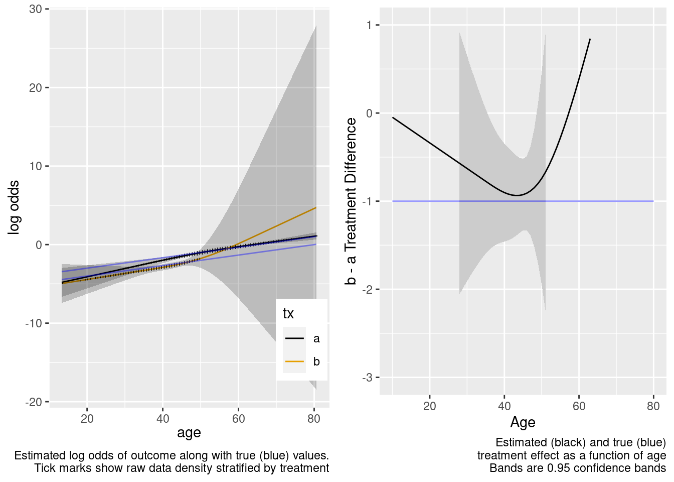
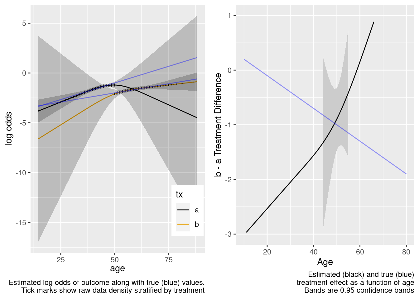
By allowing not only an unnecessary interaction but also allowing the interaction to be nonlinear, when the predicted values are for a region completely outside the sample data, the extrapolation is still reasonable but the (honest) confidence intervals are much wider. We don’t know much at all about the relative treatment effect with age < 50 when we allowed the two treatments to have differently shaped age effects in the trial data. A Bayesian model that put a skeptical prior on either the nonlinear or the interaction effect would have credible intervals that are not so wide on the left.
This model included unnecessary linear and nonlinear interaction terms.
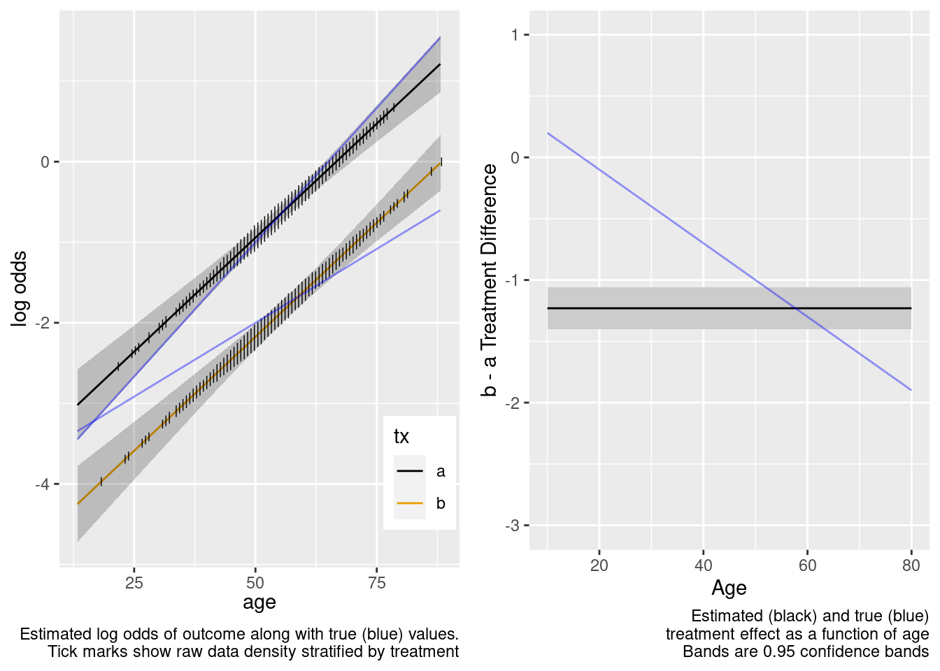
RCT Sample Partially Overlaps with Target Population
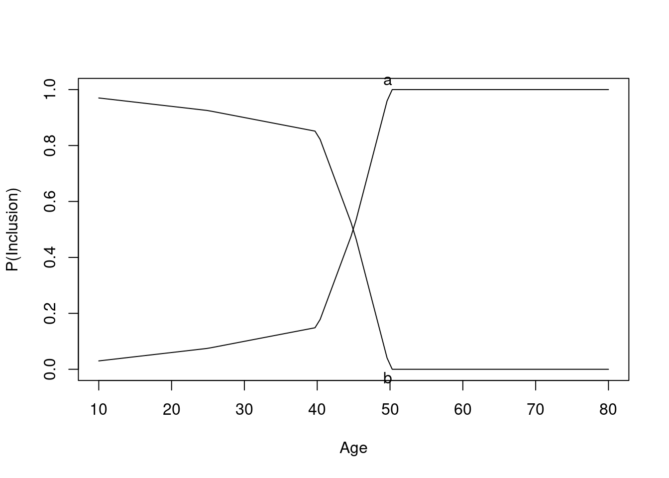
Instead of having non-overlapping age distributions between the RCT sample and the target population, let’s include screened patients with probabilities that are functions of age as shown in the first graph below. Then again consider the simplest logistic model.
The original age range is 13.3 - 88.1 in 5000 subjects, and the clinical trial includes 3556 of the subjects.
Age distributions in the target population as compared to the RCT sample are shown below.
Logistic Regression Model
lrm(formula = y ~ tx + age, data = d)
Frequencies of Missing Values Due to Each Variable
    y   tx  age
 1444    0    0
|
Model Likelihood Ratio Test |
Discrimination Indexes |
Rank Discrim. Indexes |
|
|---|---|---|---|
| Obs 3556 | LR χ2 329.69 | R2 0.131 | C 0.697 |
| 0 2658 | d.f. 2 | R22,3556 0.088 | Dxy 0.394 |
| 1 898 | Pr(>χ2) <0.0001 | R22,2013.7 0.150 | γ 0.394 |
| max |∂log L/∂β| 3×10-11 | Brier 0.171 | τa 0.149 |
| β | S.E. | Wald Z | Pr(>|Z|) | |
|---|---|---|---|---|
| Intercept | -4.4121 | 0.2941 | -15.00 | <0.0001 |
| tx=b | -1.0470 | 0.0846 | -12.38 | <0.0001 |
| age | 0.0682 | 0.0052 | 13.04 | <0.0001 |
Wald Statistics for y
|
|||
| χ2 | d.f. | P | |
|---|---|---|---|
| tx | 153.17 | 1 | <0.0001 |
| age | 169.92 | 1 | <0.0001 |
| TOTAL | 286.93 | 2 | <0.0001 |
This is the correct model.
Logistic Regression Model
lrm(formula = y ~ tx * age, data = d)
Frequencies of Missing Values Due to Each Variable
    y   tx  age
 1444    0    0
|
Model Likelihood Ratio Test |
Discrimination Indexes |
Rank Discrim. Indexes |
|
|---|---|---|---|
| Obs 3556 | LR χ2 330.73 | R2 0.131 | C 0.697 |
| 0 2658 | d.f. 3 | R23,3556 0.088 | Dxy 0.394 |
| 1 898 | Pr(>χ2) <0.0001 | R23,2013.7 0.150 | γ 0.394 |
| max |∂log L/∂β| 1×10-11 | Brier 0.171 | τa 0.149 |
| β | S.E. | Wald Z | Pr(>|Z|) | |
|---|---|---|---|---|
| Intercept | -4.6606 | 0.3849 | -12.11 | <0.0001 |
| tx=b | -0.4360 | 0.6056 | -0.72 | 0.4715 |
| age | 0.0726 | 0.0069 | 10.56 | <0.0001 |
| tx=b × age | -0.0108 | 0.0106 | -1.02 | 0.3089 |
Wald Statistics for y
|
|||
| χ2 | d.f. | P | |
|---|---|---|---|
| tx (Factor+Higher Order Factors) | 154.98 | 2 | <0.0001 |
| All Interactions | 1.04 | 1 | 0.3089 |
| age (Factor+Higher Order Factors) | 169.90 | 2 | <0.0001 |
| All Interactions | 1.04 | 1 | 0.3089 |
| tx × age (Factor+Higher Order Factors) | 1.04 | 1 | 0.3089 |
| TOTAL | 292.05 | 3 | <0.0001 |

This model included an unnecessary linear interaction term.
Logistic Regression Model
lrm(formula = form, data = d, tol = 1e-12)
Frequencies of Missing Values Due to Each Variable
    y   tx  age
 1444    0    0
|
Model Likelihood Ratio Test |
Discrimination Indexes |
Rank Discrim. Indexes |
|
|---|---|---|---|
| Obs 3556 | LR χ2 333.43 | R2 0.132 | C 0.697 |
| 0 2658 | d.f. 7 | R27,3556 0.088 | Dxy 0.395 |
| 1 898 | Pr(>χ2) <0.0001 | R27,2013.7 0.150 | γ 0.395 |
| max |∂log L/∂β| 5×10-11 | Brier 0.171 | τa 0.149 |
| β | S.E. | Wald Z | Pr(>|Z|) | |
|---|---|---|---|---|
| Intercept | -4.7933 | 0.5949 | -8.06 | <0.0001 |
| tx=b | 0.6350 | 0.9700 | 0.65 | 0.5127 |
| age | 0.0752 | 0.0113 | 6.67 | <0.0001 |
| age’ | -0.0274 | 0.1673 | -0.16 | 0.8699 |
| age’’ | 0.0392 | 0.4011 | 0.10 | 0.9221 |
| tx=b × age | -0.0319 | 0.0183 | -1.74 | 0.0820 |
| tx=b × age’ | 0.2854 | 0.2321 | 1.23 | 0.2188 |
| tx=b × age’’ | -0.5634 | 0.5254 | -1.07 | 0.2836 |
Wald Statistics for y
|
|||
| χ2 | d.f. | P | |
|---|---|---|---|
| tx (Factor+Higher Order Factors) | 155.86 | 4 | <0.0001 |
| All Interactions | 3.03 | 3 | 0.3873 |
| age (Factor+Higher Order Factors) | 175.89 | 6 | <0.0001 |
| All Interactions | 3.03 | 3 | 0.3873 |
| Nonlinear (Factor+Higher Order Factors) | 2.73 | 4 | 0.6041 |
| tx × age (Factor+Higher Order Factors) | 3.03 | 3 | 0.3873 |
| Nonlinear | 1.93 | 2 | 0.3813 |
| Nonlinear Interaction : f(A,B) vs. AB | 1.93 | 2 | 0.3813 |
| TOTAL NONLINEAR | 2.73 | 4 | 0.6041 |
| TOTAL NONLINEAR + INTERACTION | 3.82 | 5 | 0.5755 |
| TOTAL | 299.44 | 7 | <0.0001 |
This model included unnecessary linear and nonlinear interaction terms.
Case Where Treatment Truly Interacts with Age
Estimation of Treatment Effect in Population With No Overlap
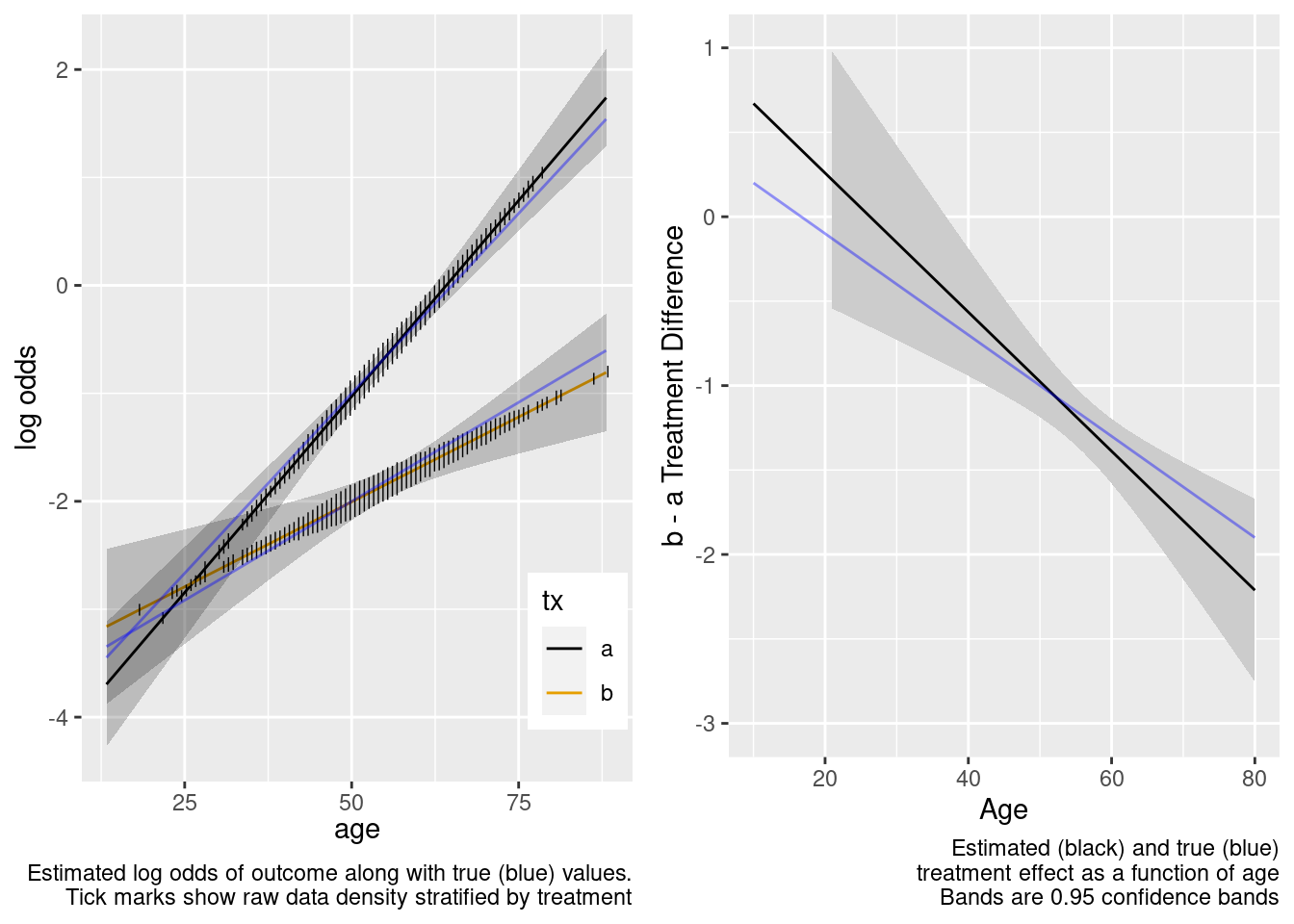
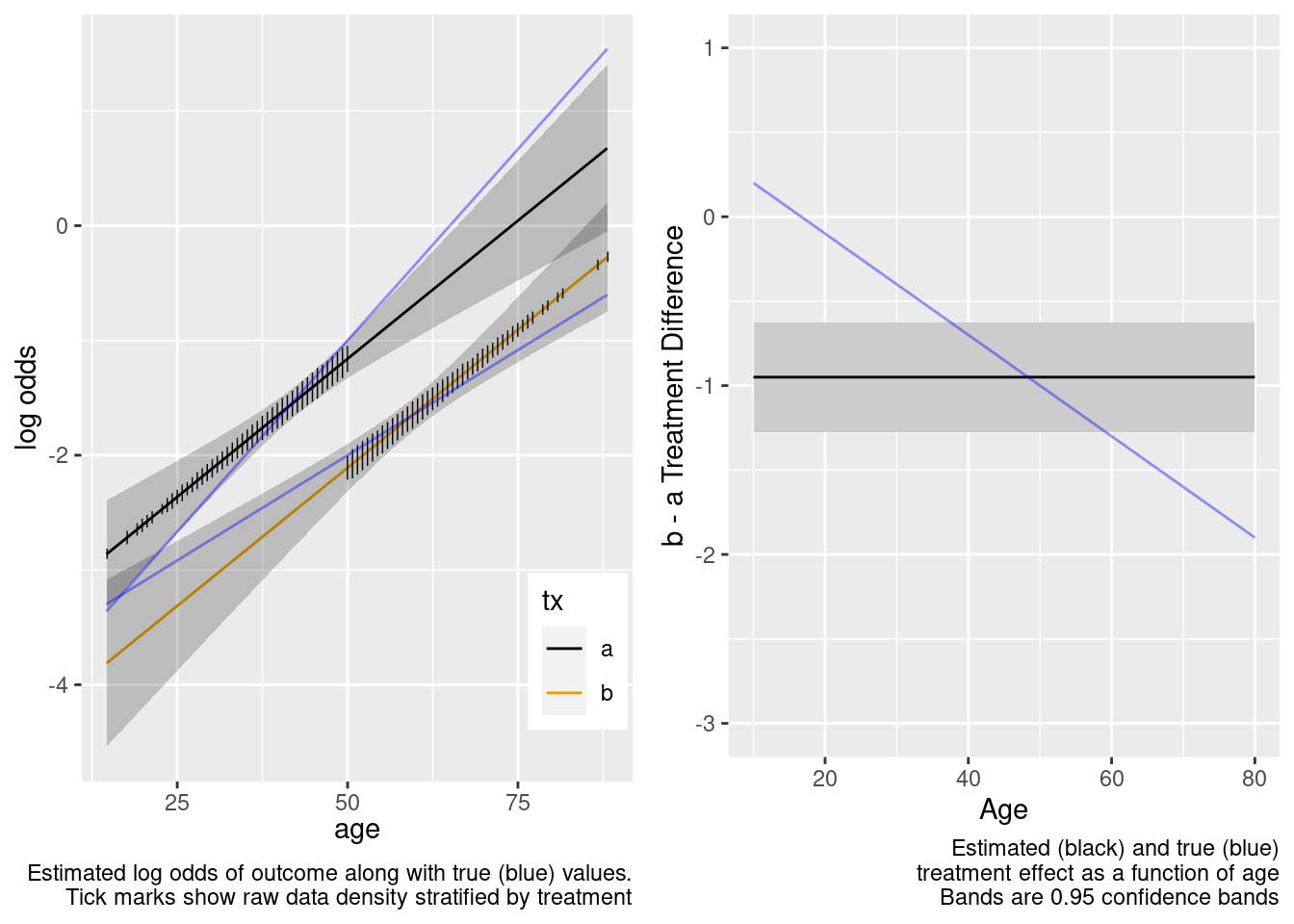
Next turn to the case where the true data generating model has a linear treatment by age interaction which we may or may not include in our model. The true model has a treatment effect of -1.0 for age 50 patients, and each year below 50 results in a further reduction by 0.03 in the effect.
Logistic Regression Model
lrm(formula = y ~ tx + age, data = d)
Frequencies of Missing Values Due to Each Variable
    y   tx  age
 2539    0    0
|
Model Likelihood Ratio Test |
Discrimination Indexes |
Rank Discrim. Indexes |
|
|---|---|---|---|
| Obs 2461 | LR χ2 257.32 | R2 0.144 | C 0.701 |
| 0 1787 | d.f. 2 | R22,2461 0.099 | Dxy 0.403 |
| 1 674 | Pr(>χ2) <0.0001 | R22,1468.2 0.160 | γ 0.403 |
| max |∂log L/∂β| 9×10⁻⁶ | Brier 0.178 | τa 0.160 |
| β | S.E. | Wald Z | Pr(>|Z|) | |
|---|---|---|---|---|
| Intercept | -3.8181 | 0.4509 | -8.47 | <0.0001 |
| tx=b | -1.4027 | 0.1020 | -13.76 | <0.0001 |
| age | 0.0583 | 0.0077 | 7.61 | <0.0001 |
Wald Statistics for y
|
|||
| χ2 | d.f. | P | |
|---|---|---|---|
| tx | 189.24 | 1 | <0.0001 |
| age | 57.92 | 1 | <0.0001 |
| TOTAL | 223.45 | 2 | <0.0001 |
This model failed to include a needed interaction term.
Logistic Regression Model
lrm(formula = y ~ tx * age, data = d)
Frequencies of Missing Values Due to Each Variable
    y   tx  age
 2539    0    0
|
Model Likelihood Ratio Test |
Discrimination Indexes |
Rank Discrim. Indexes |
|
|---|---|---|---|
| Obs 2461 | LR χ2 258.51 | R2 0.144 | C 0.702 |
| 0 1787 | d.f. 3 | R23,2461 0.099 | Dxy 0.403 |
| 1 674 | Pr(>χ2) <0.0001 | R23,1468.2 0.160 | γ 0.403 |
| max |∂log L/∂β| 2×10-12 | Brier 0.178 | τa 0.160 |
| β | S.E. | Wald Z | Pr(>|Z|) | |
|---|---|---|---|---|
| Intercept | -4.2193 | 0.5852 | -7.21 | <0.0001 |
| tx=b | -0.3879 | 0.9367 | -0.41 | 0.6788 |
| age | 0.0652 | 0.0100 | 6.53 | <0.0001 |
| tx=b × age | -0.0171 | 0.0157 | -1.09 | 0.2765 |
Wald Statistics for y
|
|||
| χ2 | d.f. | P | |
|---|---|---|---|
| tx (Factor+Higher Order Factors) | 191.47 | 2 | <0.0001 |
| All Interactions | 1.18 | 1 | 0.2765 |
| age (Factor+Higher Order Factors) | 58.35 | 2 | <0.0001 |
| All Interactions | 1.18 | 1 | 0.2765 |
| tx × age (Factor+Higher Order Factors) | 1.18 | 1 | 0.2765 |
| TOTAL | 228.30 | 3 | <0.0001 |
Because of the more limited age range in the trial there was insufficient power to provide definitive statistical evidence for an interaction, but the point estimate for the interaction effect is not unreasonable. Though confidence bands are wide because of no overlap, the extrapolated treatment effects are reasonable as a result.
This is the correct model.
Logistic Regression Model
lrm(formula = form, data = d, tol = 1e-12)
Frequencies of Missing Values Due to Each Variable
    y   tx  age
 2539    0    0
|
Model Likelihood Ratio Test |
Discrimination Indexes |
Rank Discrim. Indexes |
|
|---|---|---|---|
| Obs 2461 | LR χ2 261.24 | R2 0.146 | C 0.702 |
| 0 1787 | d.f. 7 | R27,2461 0.098 | Dxy 0.403 |
| 1 674 | Pr(>χ2) <0.0001 | R27,1468.2 0.159 | γ 0.404 |
| max |∂log L/∂β| 1×10-12 | Brier 0.178 | τa 0.161 |
| β | S.E. | Wald Z | Pr(>|Z|) | |
|---|---|---|---|---|
| Intercept | -3.0988 | 1.2779 | -2.42 | 0.0153 |
| tx=b | 0.1305 | 2.1946 | 0.06 | 0.9526 |
| age | 0.0445 | 0.0231 | 1.93 | 0.0542 |
| age’ | 0.2124 | 0.2213 | 0.96 | 0.3372 |
| age’’ | -0.4384 | 0.4906 | -0.89 | 0.3716 |
| tx=b × age | -0.0267 | 0.0396 | -0.68 | 0.4996 |
| tx=b × age’ | 0.0955 | 0.3313 | 0.29 | 0.7731 |
| tx=b × age’’ | -0.1934 | 0.6939 | -0.28 | 0.7805 |
Wald Statistics for y
|
|||
| χ2 | d.f. | P | |
|---|---|---|---|
| tx (Factor+Higher Order Factors) | 191.14 | 4 | <0.0001 |
| All Interactions | 1.19 | 3 | 0.7545 |
| age (Factor+Higher Order Factors) | 61.60 | 6 | <0.0001 |
| All Interactions | 1.19 | 3 | 0.7545 |
| Nonlinear (Factor+Higher Order Factors) | 2.67 | 4 | 0.6150 |
| tx × age (Factor+Higher Order Factors) | 1.19 | 3 | 0.7545 |
| Nonlinear | 0.08 | 2 | 0.9590 |
| Nonlinear Interaction : f(A,B) vs. AB | 0.08 | 2 | 0.9590 |
| TOTAL NONLINEAR | 2.67 | 4 | 0.6150 |
| TOTAL NONLINEAR + INTERACTION | 3.78 | 5 | 0.5816 |
| TOTAL | 229.68 | 7 | <0.0001 |
This model correctly captures linear interaction, but also allows for unnecessary nonlinear interaction.
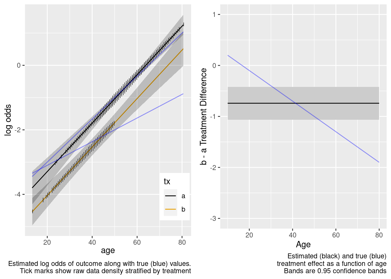
RCT Sample Partially Overlaps with Target Population
Sticking with the true treatment effect interacting with age, we generate data with the same partial overlap as before, and repeat the same analyses. We start by fitting a model that is oblivious to interaction.
Logistic Regression Model
lrm(formula = y ~ tx + age, data = d)
Frequencies of Missing Values Due to Each Variable
    y   tx  age
 1444    0    0
|
Model Likelihood Ratio Test |
Discrimination Indexes |
Rank Discrim. Indexes |
|
|---|---|---|---|
| Obs 3556 | LR χ2 323.95 | R2 0.130 | C 0.699 |
| 0 2702 | d.f. 2 | R22,3556 0.087 | Dxy 0.397 |
| 1 854 | Pr(>χ2) <0.0001 | R22,1946.7 0.152 | γ 0.397 |
| max |∂log L/∂β| 8×10-12 | Brier 0.165 | τa 0.145 |
| β | S.E. | Wald Z | Pr(>|Z|) | |
|---|---|---|---|---|
| Intercept | -3.7735 | 0.2939 | -12.84 | <0.0001 |
| tx=b | -1.2305 | 0.0876 | -14.04 | <0.0001 |
| age | 0.0566 | 0.0052 | 10.80 | <0.0001 |
Wald Statistics for y
|
|||
| χ2 | d.f. | P | |
|---|---|---|---|
| tx | 197.20 | 1 | <0.0001 |
| age | 116.73 | 1 | <0.0001 |
| TOTAL | 281.79 | 2 | <0.0001 |
This model failed to include a needed interaction term.
Logistic Regression Model
lrm(formula = y ~ tx * age, data = d)
Frequencies of Missing Values Due to Each Variable
    y   tx  age
 1444    0    0
|
Model Likelihood Ratio Test |
Discrimination Indexes |
Rank Discrim. Indexes |
|
|---|---|---|---|
| Obs 3556 | LR χ2 338.39 | R2 0.136 | C 0.700 |
| 0 2702 | d.f. 3 | R23,3556 0.090 | Dxy 0.400 |
| 1 854 | Pr(>χ2) <0.0001 | R23,1946.7 0.158 | γ 0.401 |
| max |∂log L/∂β| 3×10-12 | Brier 0.164 | τa 0.146 |
| β | S.E. | Wald Z | Pr(>|Z|) | |
|---|---|---|---|---|
| Intercept | -4.6606 | 0.3849 | -12.11 | <0.0001 |
| tx=b | 1.0820 | 0.6129 | 1.77 | 0.0775 |
| age | 0.0726 | 0.0069 | 10.56 | <0.0001 |
| tx=b × age | -0.0412 | 0.0109 | -3.79 | 0.0002 |
Wald Statistics for y
|
|||
| χ2 | d.f. | P | |
|---|---|---|---|
| tx (Factor+Higher Order Factors) | 210.59 | 2 | <0.0001 |
| All Interactions | 14.36 | 1 | 0.0002 |
| age (Factor+Higher Order Factors) | 125.47 | 2 | <0.0001 |
| All Interactions | 14.36 | 1 | 0.0002 |
| tx × age (Factor+Higher Order Factors) | 14.36 | 1 | 0.0002 |
| TOTAL | 310.44 | 3 | <0.0001 |
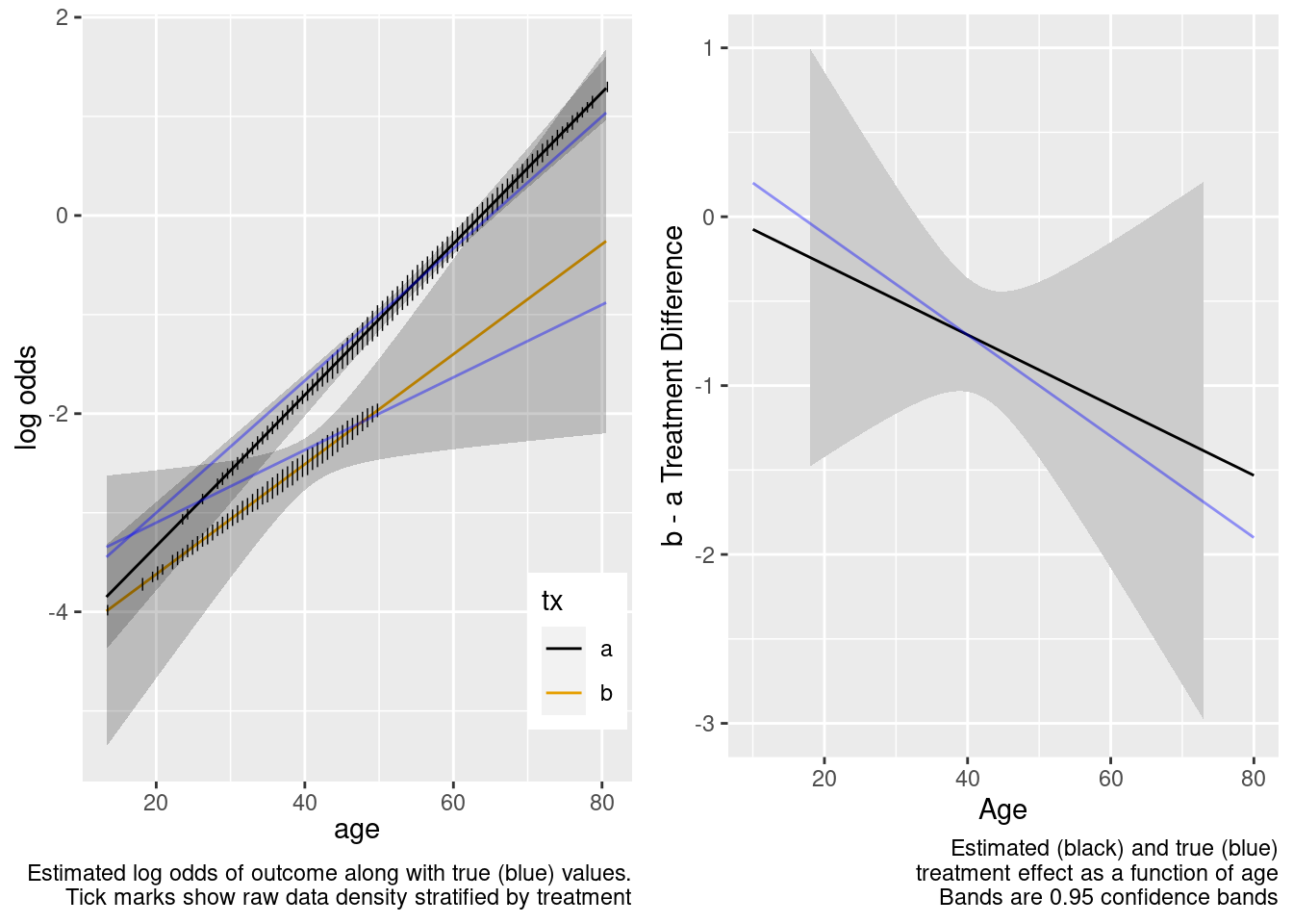
The amount of interaction estimated from the larger older sample extrapolated well to the younger target population.
This is the correct model.
Logistic Regression Model
lrm(formula = form, data = d, tol = 1e-12)
Frequencies of Missing Values Due to Each Variable
    y   tx  age
 1444    0    0
|
Model Likelihood Ratio Test |
Discrimination Indexes |
Rank Discrim. Indexes |
|
|---|---|---|---|
| Obs 3556 | LR χ2 343.94 | R2 0.138 | C 0.700 |
| 0 2702 | d.f. 7 | R27,3556 0.090 | Dxy 0.401 |
| 1 854 | Pr(>χ2) <0.0001 | R27,1946.7 0.159 | γ 0.401 |
| max |∂log L/∂β| 7×10-12 | Brier 0.164 | τa 0.146 |
| β | S.E. | Wald Z | Pr(>|Z|) | |
|---|---|---|---|---|
| Intercept | -4.7933 | 0.5949 | -8.06 | <0.0001 |
| tx=b | 2.5181 | 0.9368 | 2.69 | 0.0072 |
| age | 0.0752 | 0.0113 | 6.67 | <0.0001 |
| age’ | -0.0274 | 0.1673 | -0.16 | 0.8699 |
| age’’ | 0.0392 | 0.4011 | 0.10 | 0.9221 |
| tx=b × age | -0.0698 | 0.0179 | -3.91 | <0.0001 |
| tx=b × age’ | 0.4148 | 0.2398 | 1.73 | 0.0836 |
| tx=b × age’’ | -0.8163 | 0.5469 | -1.49 | 0.1355 |
Wald Statistics for y
|
|||
| χ2 | d.f. | P | |
|---|---|---|---|
| tx (Factor+Higher Order Factors) | 211.50 | 4 | <0.0001 |
| All Interactions | 19.06 | 3 | 0.0003 |
| age (Factor+Higher Order Factors) | 132.65 | 6 | <0.0001 |
| All Interactions | 19.06 | 3 | 0.0003 |
| Nonlinear (Factor+Higher Order Factors) | 5.66 | 4 | 0.2263 |
| tx × age (Factor+Higher Order Factors) | 19.06 | 3 | 0.0003 |
| Nonlinear | 3.97 | 2 | 0.1374 |
| Nonlinear Interaction : f(A,B) vs. AB | 3.97 | 2 | 0.1374 |
| TOTAL NONLINEAR | 5.66 | 4 | 0.2263 |
| TOTAL NONLINEAR + INTERACTION | 20.91 | 5 | 0.0008 |
| TOTAL | 316.28 | 7 | <0.0001 |
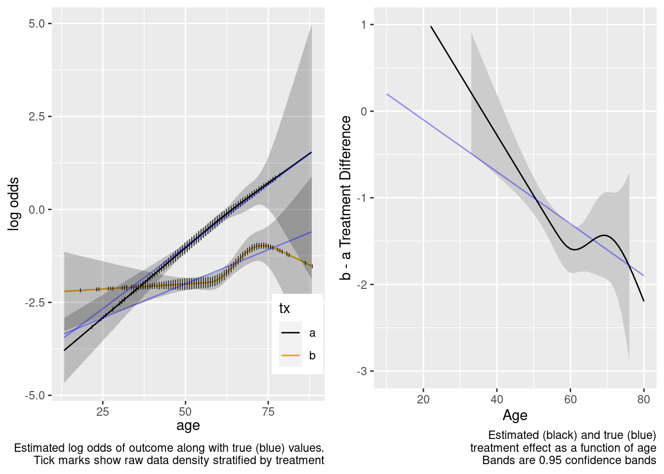
The spline interaction estimates did not extrapolate well to the very young.
This model correctly captures linear interaction, but also allows for unnecessary nonlinear interaction.
Ability to Compare Treatments in Observational Studies
When a categorical baseline characteristic has all of the patients in one of its categories getting a single treatment, one cannot estimate efficacy in that category unless (1) there is no interaction between treatment and the variable or (2) the baseline variable does not relate to outcome. If one of these conditions is not satisfied, one would have to do a conditional analysis, i.e., to estimate efficacy in patients not in the offending category. If a continuous baseline variable has an interval for which every patient in that interval received only one treatment, then one cannot estimate the treatment effect in that interval unless (1) there is no interaction (linear or nonlinear) between the variable and treatment or (2) the variable is irrelevant to outcome. So when you hear that non-overlap implies that only a conditional treatment comparison can be done, be aware of the true underlying assumptions. Note that non-overlap on a variable implies non-overlap for one or more values of a propensity score.
To illustrate these points, consider an observational study where the data generating process is from the same population logistic model as used above, but instead of considering generalizability to a population, consider the in-sample comparison of treatments a and b adjusted for age. We start with a sample in which all those with age ≥ 50 got treatment b and all those with age < 50 got treatment a.
True Model Has No Treatment Interactions
No Overlap Between Treatment Groups
All patients age < 50 had treatment a, and those ≥ 50 had b.
Age distributions in the observed treatment groups are shown below.
Logistic Regression Model
lrm(formula = y ~ tx + age, data = d)
|
Model Likelihood Ratio Test |
Discrimination Indexes |
Rank Discrim. Indexes |
|
|---|---|---|---|
| Obs 2999 | LR χ2 87.42 | R2 0.046 | C 0.616 |
| 0 2431 | d.f. 2 | R22,2999 0.028 | Dxy 0.232 |
| 1 568 | Pr(>χ2) <0.0001 | R22,1381.3 0.060 | γ 0.232 |
| max |∂log L/∂β| 8×10⁻⁹ | Brier 0.149 | τa 0.071 |
| β | S.E. | Wald Z | Pr(>|Z|) | |
|---|---|---|---|---|
| Intercept | -4.5743 | 0.3532 | -12.95 | <0.0001 |
| tx=b | -1.0283 | 0.1608 | -6.40 | <0.0001 |
| age | 0.0714 | 0.0080 | 8.96 | <0.0001 |
Wald Statistics for y
|
|||
| χ2 | d.f. | P | |
|---|---|---|---|
| tx | 40.90 | 1 | <0.0001 |
| age | 80.26 | 1 | <0.0001 |
| TOTAL | 82.33 | 2 | <0.0001 |
The model-based covariate adjustment provided the correct estimate of the treatment effect even with no overlap, since the specified model is the correct model.
This is the correct model.
Logistic Regression Model
lrm(formula = y ~ tx * age, data = d)
|
Model Likelihood Ratio Test |
Discrimination Indexes |
Rank Discrim. Indexes |
|
|---|---|---|---|
| Obs 2999 | LR χ2 88.00 | R2 0.047 | C 0.616 |
| 0 2431 | d.f. 3 | R23,2999 0.028 | Dxy 0.231 |
| 1 568 | Pr(>χ2) <0.0001 | R23,1381.3 0.060 | γ 0.232 |
| max |∂log L/∂β| 5×10⁻⁷ | Brier 0.149 | τa 0.071 |
| β | S.E. | Wald Z | Pr(>|Z|) | |
|---|---|---|---|---|
| Intercept | -4.2550 | 0.5399 | -7.88 | <0.0001 |
| tx=b | -1.6471 | 0.8237 | -2.00 | 0.0455 |
| age | 0.0641 | 0.0124 | 5.19 | <0.0001 |
| tx=b × age | 0.0124 | 0.0161 | 0.77 | 0.4430 |
Wald Statistics for y
|
|||
| χ2 | d.f. | P | |
|---|---|---|---|
| tx (Factor+Higher Order Factors) | 40.98 | 2 | <0.0001 |
| All Interactions | 0.59 | 1 | 0.4430 |
| age (Factor+Higher Order Factors) | 81.73 | 2 | <0.0001 |
| All Interactions | 0.59 | 1 | 0.4430 |
| tx × age (Factor+Higher Order Factors) | 0.59 | 1 | 0.4430 |
| TOTAL | 84.33 | 3 | <0.0001 |
With no age overlap, the treatment by age interaction is estimated very inefficiently and in this case incorrectly. Wide confidence bands correctly capture the difficulty of the task of estimating age-specific treatment effects.
This model included an unnecessary linear interaction term.
Logistic Regression Model
lrm(formula = form, data = d, tol = 1e-12)
|
Model Likelihood Ratio Test |
Discrimination Indexes |
Rank Discrim. Indexes |
|
|---|---|---|---|
| Obs 2999 | LR χ2 89.34 | R2 0.047 | C 0.617 |
| 0 2431 | d.f. 5 | R25,2999 0.028 | Dxy 0.233 |
| 1 568 | Pr(>χ2) <0.0001 | R25,1381.3 0.059 | γ 0.234 |
| max |∂log L/∂β| 7×10-12 | Brier 0.149 | τa 0.072 |
| β | S.E. | Wald Z | Pr(>|Z|) | |
|---|---|---|---|---|
| Intercept | -5.0833 | 0.9349 | -5.44 | <0.0001 |
| tx=b | 0.4348 | 7.1719 | 0.06 | 0.9517 |
| age | 0.0868 | 0.0241 | 3.60 | 0.0003 |
| age’ | -0.1233 | 0.1090 | -1.13 | 0.2580 |
| tx=b × age | -0.0361 | 0.1482 | -0.24 | 0.8073 |
| tx=b × age’ | 0.1420 | 0.1520 | 0.93 | 0.3502 |
Wald Statistics for y
|
|||
| χ2 | d.f. | P | |
|---|---|---|---|
| tx (Factor+Higher Order Factors) | 40.98 | 3 | <0.0001 |
| All Interactions | 1.50 | 2 | 0.4734 |
| age (Factor+Higher Order Factors) | 80.92 | 4 | <0.0001 |
| All Interactions | 1.50 | 2 | 0.4734 |
| Nonlinear (Factor+Higher Order Factors) | 1.31 | 2 | 0.5193 |
| tx × age (Factor+Higher Order Factors) | 1.50 | 2 | 0.4734 |
| Nonlinear | 0.87 | 1 | 0.3502 |
| Nonlinear Interaction : f(A,B) vs. AB | 0.87 | 1 | 0.3502 |
| TOTAL NONLINEAR | 1.31 | 2 | 0.5193 |
| TOTAL NONLINEAR + INTERACTION | 1.90 | 3 | 0.5925 |
| TOTAL | 83.33 | 5 | <0.0001 |
This model included unnecessary linear and nonlinear interaction terms.
Some Overlap in Ages Between Treatments
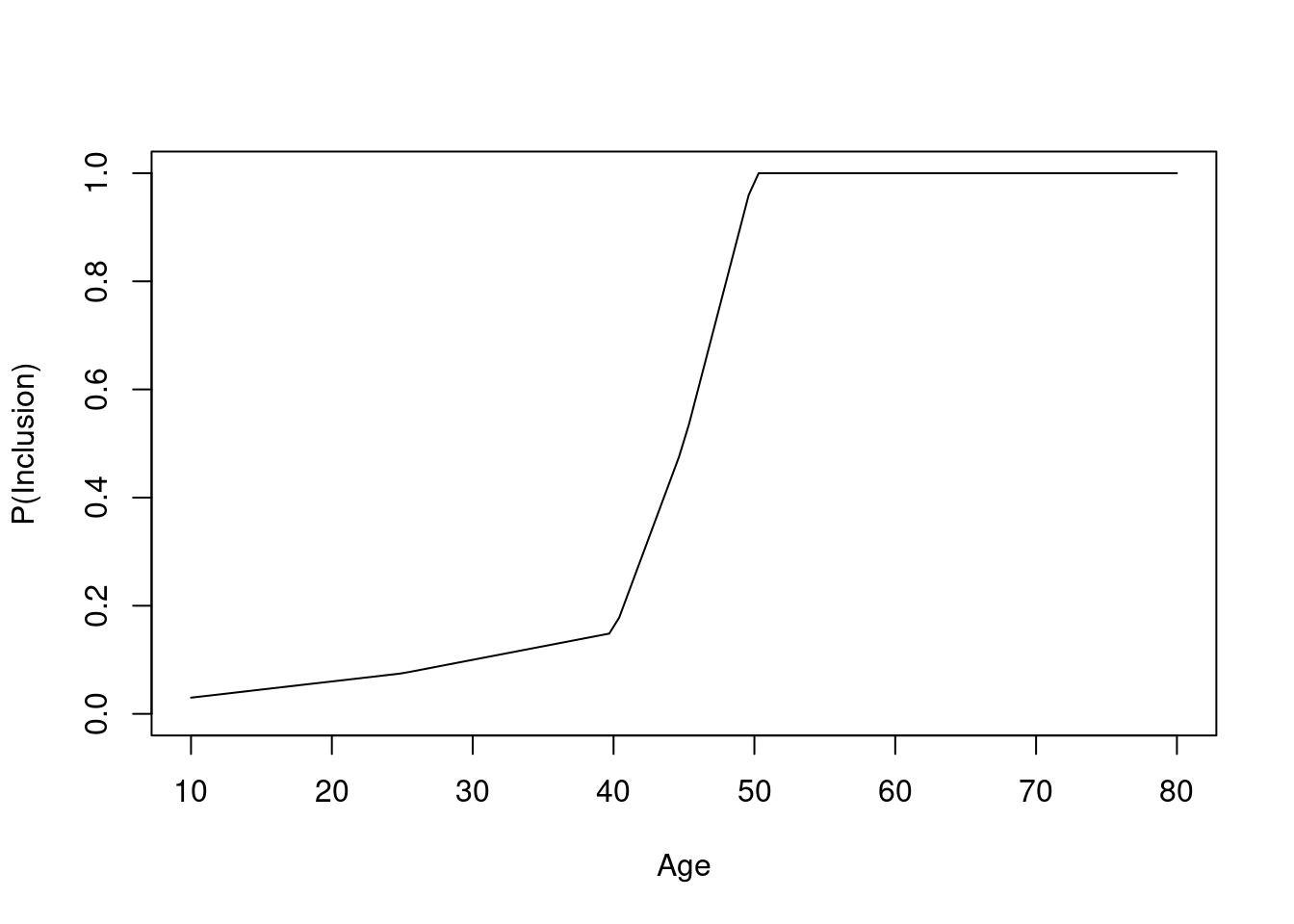
Now consider an observational study, again with confounding by indication, related to age. Partial overlap is defined by specifying separate study inclusion probability functions. Given the age and treatment these functions specify the probability that a patient would be included in the observational study. The first plot shows the inclusion probabilities separately for treatments a and b. Then the result of a linear no-interaction model are shown. As before, blue curves depict true data-generating model log odds.
The graph below shows the probability of selection into each of the observed treatment groups as a function of age.
Age distributions in the observed treatment groups are shown below.
Logistic Regression Model
lrm(formula = y ~ tx + age, data = d)
|
Model Likelihood Ratio Test |
Discrimination Indexes |
Rank Discrim. Indexes |
|
|---|---|---|---|
| Obs 3031 | LR χ2 474.99 | R2 0.212 | C 0.744 |
| 0 2236 | d.f. 2 | R22,3031 0.144 | Dxy 0.488 |
| 1 795 | Pr(>χ2) <0.0001 | R22,1759.4 0.236 | γ 0.489 |
| max |∂log L/∂β| 9×10⁻⁶ | Brier 0.166 | τa 0.189 |
| β | S.E. | Wald Z | Pr(>|Z|) | |
|---|---|---|---|---|
| Intercept | -4.8959 | 0.3443 | -14.22 | <0.0001 |
| tx=b | -1.0104 | 0.1787 | -5.65 | <0.0001 |
| age | 0.0769 | 0.0061 | 12.53 | <0.0001 |
Wald Statistics for y
|
|||
| χ2 | d.f. | P | |
|---|---|---|---|
| tx | 31.98 | 1 | <0.0001 |
| age | 156.93 | 1 | <0.0001 |
| TOTAL | 335.25 | 2 | <0.0001 |
This is the correct model.
Logistic Regression Model
lrm(formula = y ~ tx * age, data = d)
|
Model Likelihood Ratio Test |
Discrimination Indexes |
Rank Discrim. Indexes |
|
|---|---|---|---|
| Obs 3031 | LR χ2 475.20 | R2 0.212 | C 0.744 |
| 0 2236 | d.f. 3 | R23,3031 0.144 | Dxy 0.488 |
| 1 795 | Pr(>χ2) <0.0001 | R23,1759.4 0.235 | γ 0.489 |
| max |∂log L/∂β| 1×10⁻⁸ | Brier 0.166 | τa 0.189 |
| β | S.E. | Wald Z | Pr(>|Z|) | |
|---|---|---|---|---|
| Intercept | -4.8638 | 0.3512 | -13.85 | <0.0001 |
| tx=b | -1.6044 | 1.3432 | -1.19 | 0.2323 |
| age | 0.0763 | 0.0063 | 12.18 | <0.0001 |
| tx=b × age | 0.0141 | 0.0314 | 0.45 | 0.6546 |
Wald Statistics for y
|
|||
| χ2 | d.f. | P | |
|---|---|---|---|
| tx (Factor+Higher Order Factors) | 32.33 | 2 | <0.0001 |
| All Interactions | 0.20 | 1 | 0.6546 |
| age (Factor+Higher Order Factors) | 157.04 | 2 | <0.0001 |
| All Interactions | 0.20 | 1 | 0.6546 |
| tx × age (Factor+Higher Order Factors) | 0.20 | 1 | 0.6546 |
| TOTAL | 330.68 | 3 | <0.0001 |
The confidence bands are correctly registering that there is little information about the treatment effect outside of the heavier overlap region.
This model included an unnecessary linear interaction term.
Logistic Regression Model
lrm(formula = form, data = d, tol = 1e-12)
|
Model Likelihood Ratio Test |
Discrimination Indexes |
Rank Discrim. Indexes |
|
|---|---|---|---|
| Obs 3031 | LR χ2 476.54 | R2 0.213 | C 0.744 |
| 0 2236 | d.f. 5 | R25,3031 0.144 | Dxy 0.489 |
| 1 795 | Pr(>χ2) <0.0001 | R25,1759.4 0.235 | γ 0.489 |
| max |∂log L/∂β| 2×10⁻⁷ | Brier 0.166 | τa 0.189 |
| β | S.E. | Wald Z | Pr(>|Z|) | |
|---|---|---|---|---|
| Intercept | -6.2165 | 1.3037 | -4.77 | <0.0001 |
| tx=b | 0.2424 | 2.3347 | 0.10 | 0.9173 |
| age | 0.1058 | 0.0280 | 3.78 | 0.0002 |
| age’ | -0.0262 | 0.0240 | -1.09 | 0.2761 |
| tx=b × age | -0.0291 | 0.0579 | -0.50 | 0.6155 |
| tx=b × age’ | 0.1247 | 0.2974 | 0.42 | 0.6749 |
Wald Statistics for y
|
|||
| χ2 | d.f. | P | |
|---|---|---|---|
| tx (Factor+Higher Order Factors) | 20.25 | 3 | 0.0002 |
| All Interactions | 0.26 | 2 | 0.8794 |
| age (Factor+Higher Order Factors) | 154.87 | 4 | <0.0001 |
| All Interactions | 0.26 | 2 | 0.8794 |
| Nonlinear (Factor+Higher Order Factors) | 1.30 | 2 | 0.5229 |
| tx × age (Factor+Higher Order Factors) | 0.26 | 2 | 0.8794 |
| Nonlinear | 0.18 | 1 | 0.6749 |
| Nonlinear Interaction : f(A,B) vs. AB | 0.18 | 1 | 0.6749 |
| TOTAL NONLINEAR | 1.30 | 2 | 0.5229 |
| TOTAL NONLINEAR + INTERACTION | 1.51 | 3 | 0.6793 |
| TOTAL | 330.06 | 5 | <0.0001 |
This model included unnecessary linear and nonlinear interaction terms.
Case Where Treatment Truly Interacts with Age
No Overlap Between Treatment Groups
Return to the data generating model used in the RCT simulation, for which there is truly a linear interaction with treatment, and start with the no overlap case.
Logistic Regression Model
lrm(formula = y ~ tx + age, data = d)
|
Model Likelihood Ratio Test |
Discrimination Indexes |
Rank Discrim. Indexes |
|
|---|---|---|---|
| Obs 2999 | LR χ2 39.09 | R2 0.022 | C 0.591 |
| 0 2493 | d.f. 2 | R22,2999 0.012 | Dxy 0.181 |
| 1 506 | Pr(>χ2) <0.0001 | R22,1261.9 0.029 | γ 0.181 |
| max |∂log L/∂β| 4×10-11 | Brier 0.139 | τa 0.051 |
| β | S.E. | Wald Z | Pr(>|Z|) | |
|---|---|---|---|---|
| Intercept | -3.5659 | 0.3538 | -10.08 | <0.0001 |
| tx=b | -0.9499 | 0.1661 | -5.72 | <0.0001 |
| age | 0.0481 | 0.0081 | 5.96 | <0.0001 |
Wald Statistics for y
|
|||
| χ2 | d.f. | P | |
|---|---|---|---|
| tx | 32.71 | 1 | <0.0001 |
| age | 35.51 | 1 | <0.0001 |
| TOTAL | 37.94 | 2 | <0.0001 |
The treatment effect is incorrect example at age=50.
This model failed to include a needed interaction term.
Logistic Regression Model
lrm(formula = y ~ tx * age, data = d)
|
Model Likelihood Ratio Test |
Discrimination Indexes |
Rank Discrim. Indexes |
|
|---|---|---|---|
| Obs 2999 | LR χ2 42.28 | R2 0.023 | C 0.592 |
| 0 2493 | d.f. 3 | R23,2999 0.013 | Dxy 0.184 |
| 1 506 | Pr(>χ2) <0.0001 | R23,1261.9 0.031 | γ 0.185 |
| max |∂log L/∂β| 3×10⁻⁸ | Brier 0.138 | τa 0.052 |
| β | S.E. | Wald Z | Pr(>|Z|) | |
|---|---|---|---|---|
| Intercept | -4.2550 | 0.5399 | -7.88 | <0.0001 |
| tx=b | 0.5441 | 0.8578 | 0.63 | 0.5259 |
| age | 0.0641 | 0.0124 | 5.19 | <0.0001 |
| tx=b × age | -0.0295 | 0.0167 | -1.77 | 0.0767 |
Wald Statistics for y
|
|||
| χ2 | d.f. | P | |
|---|---|---|---|
| tx (Factor+Higher Order Factors) | 36.26 | 2 | <0.0001 |
| All Interactions | 3.13 | 1 | 0.0767 |
| age (Factor+Higher Order Factors) | 36.45 | 2 | <0.0001 |
| All Interactions | 3.13 | 1 | 0.0767 |
| tx × age (Factor+Higher Order Factors) | 3.13 | 1 | 0.0767 |
| TOTAL | 40.05 | 3 | <0.0001 |
The extrapolation is excellent. Now try the overkill model.
This is the correct model.
Logistic Regression Model
lrm(formula = form, data = d, tol = 1e-12)
|
Model Likelihood Ratio Test |
Discrimination Indexes |
Rank Discrim. Indexes |
|
|---|---|---|---|
| Obs 2999 | LR χ2 44.02 | R2 0.024 | C 0.592 |
| 0 2493 | d.f. 5 | R25,2999 0.013 | Dxy 0.184 |
| 1 506 | Pr(>χ2) <0.0001 | R25,1261.9 0.030 | γ 0.185 |
| max |∂log L/∂β| 2×10⁻⁵ | Brier 0.138 | τa 0.052 |
| β | S.E. | Wald Z | Pr(>|Z|) | |
|---|---|---|---|---|
| Intercept | -5.0833 | 0.9349 | -5.44 | <0.0001 |
| tx=b | -3.5002 | 7.5833 | -0.46 | 0.6444 |
| age | 0.0868 | 0.0241 | 3.60 | 0.0003 |
| age’ | -0.1233 | 0.1090 | -1.13 | 0.2580 |
| tx=b × age | 0.0483 | 0.1568 | 0.31 | 0.7581 |
| tx=b × age’ | 0.0498 | 0.1569 | 0.32 | 0.7508 |
Wald Statistics for y
|
|||
| χ2 | d.f. | P | |
|---|---|---|---|
| tx (Factor+Higher Order Factors) | 32.65 | 3 | <0.0001 |
| All Interactions | 0.97 | 2 | 0.6143 |
| age (Factor+Higher Order Factors) | 35.52 | 4 | <0.0001 |
| All Interactions | 0.97 | 2 | 0.6143 |
| Nonlinear (Factor+Higher Order Factors) | 1.70 | 2 | 0.4269 |
| tx × age (Factor+Higher Order Factors) | 0.97 | 2 | 0.6143 |
| Nonlinear | 0.10 | 1 | 0.7508 |
| Nonlinear Interaction : f(A,B) vs. AB | 0.10 | 1 | 0.7508 |
| TOTAL NONLINEAR | 1.70 | 2 | 0.4269 |
| TOTAL NONLINEAR + INTERACTION | 4.59 | 3 | 0.2041 |
| TOTAL | 39.24 | 5 | <0.0001 |
Extrapolation failed, and the failure was thankfully signaled by very wide confidence bands for age-specific treatment effects.
This model correctly captures linear interaction, but also allows for unnecessary nonlinear interaction.
Some Overlap in Ages Between Treatments
Logistic Regression Model
lrm(formula = y ~ tx + age, data = d)
|
Model Likelihood Ratio Test |
Discrimination Indexes |
Rank Discrim. Indexes |
|
|---|---|---|---|
| Obs 3031 | LR χ2 421.49 | R2 0.189 | C 0.732 |
| 0 2221 | d.f. 2 | R22,3031 0.129 | Dxy 0.464 |
| 1 810 | Pr(>χ2) <0.0001 | R22,1780.6 0.210 | γ 0.464 |
| max |∂log L/∂β| 1×10⁻⁷ | Brier 0.170 | τa 0.182 |
| β | S.E. | Wald Z | Pr(>|Z|) | |
|---|---|---|---|---|
| Intercept | -4.7976 | 0.3406 | -14.09 | <0.0001 |
| tx=b | -0.7412 | 0.1640 | -4.52 | <0.0001 |
| age | 0.0751 | 0.0061 | 12.37 | <0.0001 |
Wald Statistics for y
|
|||
| χ2 | d.f. | P | |
|---|---|---|---|
| tx | 20.41 | 1 | <0.0001 |
| age | 153.01 | 1 | <0.0001 |
| TOTAL | 319.21 | 2 | <0.0001 |
The no-interaction model missed the boat. Now fit the correct linear interaction model.
This model failed to include a needed interaction term.
Logistic Regression Model
lrm(formula = y ~ tx * age, data = d)
|
Model Likelihood Ratio Test |
Discrimination Indexes |
Rank Discrim. Indexes |
|
|---|---|---|---|
| Obs 3031 | LR χ2 422.14 | R2 0.189 | C 0.732 |
| 0 2221 | d.f. 3 | R23,3031 0.129 | Dxy 0.464 |
| 1 810 | Pr(>χ2) <0.0001 | R23,1780.6 0.210 | γ 0.464 |
| max |∂log L/∂β| 1×10⁻⁵ | Brier 0.170 | τa 0.182 |
| β | S.E. | Wald Z | Pr(>|Z|) | |
|---|---|---|---|---|
| Intercept | -4.8638 | 0.3512 | -13.85 | <0.0001 |
| tx=b | 0.1333 | 1.0813 | 0.12 | 0.9019 |
| age | 0.0763 | 0.0063 | 12.18 | <0.0001 |
| tx=b × age | -0.0208 | 0.0255 | -0.81 | 0.4151 |
Wald Statistics for y
|
|||
| χ2 | d.f. | P | |
|---|---|---|---|
| tx (Factor+Higher Order Factors) | 20.56 | 2 | <0.0001 |
| All Interactions | 0.66 | 1 | 0.4151 |
| age (Factor+Higher Order Factors) | 153.46 | 2 | <0.0001 |
| All Interactions | 0.66 | 1 | 0.4151 |
| tx × age (Factor+Higher Order Factors) | 0.66 | 1 | 0.4151 |
| TOTAL | 326.02 | 3 | <0.0001 |
There is reasonable extrapolation. Now for the overkill model.
This is the correct model.
Logistic Regression Model
lrm(formula = form, data = d, tol = 1e-12)
|
Model Likelihood Ratio Test |
Discrimination Indexes |
Rank Discrim. Indexes |
|
|---|---|---|---|
| Obs 3031 | LR χ2 423.48 | R2 0.190 | C 0.732 |
| 0 2221 | d.f. 5 | R25,3031 0.129 | Dxy 0.464 |
| 1 810 | Pr(>χ2) <0.0001 | R25,1780.6 0.209 | γ 0.464 |
| max |∂log L/∂β| 3×10⁻⁵ | Brier 0.170 | τa 0.182 |
| β | S.E. | Wald Z | Pr(>|Z|) | |
|---|---|---|---|---|
| Intercept | -6.2165 | 1.3037 | -4.77 | <0.0001 |
| tx=b | 1.8369 | 1.9527 | 0.94 | 0.3468 |
| age | 0.1058 | 0.0280 | 3.78 | 0.0002 |
| age’ | -0.0262 | 0.0240 | -1.09 | 0.2761 |
| tx=b × age | -0.0602 | 0.0477 | -1.26 | 0.2067 |
| tx=b × age’ | 0.1114 | 0.2592 | 0.43 | 0.6672 |
Wald Statistics for y
|
|||
| χ2 | d.f. | P | |
|---|---|---|---|
| tx (Factor+Higher Order Factors) | 16.32 | 3 | 0.0010 |
| All Interactions | 1.94 | 2 | 0.3784 |
| age (Factor+Higher Order Factors) | 151.01 | 4 | <0.0001 |
| All Interactions | 1.94 | 2 | 0.3784 |
| Nonlinear (Factor+Higher Order Factors) | 1.30 | 2 | 0.5233 |
| tx × age (Factor+Higher Order Factors) | 1.94 | 2 | 0.3784 |
| Nonlinear | 0.18 | 1 | 0.6672 |
| Nonlinear Interaction : f(A,B) vs. AB | 0.18 | 1 | 0.6672 |
| TOTAL NONLINEAR | 1.30 | 2 | 0.5233 |
| TOTAL NONLINEAR + INTERACTION | 1.98 | 3 | 0.5774 |
| TOTAL | 325.31 | 5 | <0.0001 |
Extrapolated treatment effect estimates are so-so.
This model correctly captures linear interaction, but also allows for unnecessary nonlinear interaction.
Summary
With respect to relative efficacy (or both relative and absolute efficacy for continuous repsonse variables), clinical trials do not require having a representative sample of the target clinical population if there are no interactions with treatment. If there are interactions, let M denote the levels of interacting factors that are well represented in the target population. In our examples, M represents younger patients. Even with interaction present, the randomized trial still does not need to be on a representative patient sample if either (1) the trial sample is representative with respect to M (in which case omitting interactions from the model is not fatal), or (2) there is just enough representation in the sample with respect to M, and those interacting factors are appropriately modeled in the randomized trial. Unless M is richly represented in the trial, using statistical testing to decide on which interactions to include in the model is not advised, due to low power of such interaction tests. Suspected interactions, even statistically weak ones, should be included in the model when some degree of extrapolation is sought. When M is very poorly represented in the trial, extrapolation to the target population makes strong model assumptions. Thankfully confidence intervals for extrapolated efficacy estimates will be properly wide to reflect the weak basis for such extrapolation.
In a similar vein, observational treatment comparisons can be appropriate if factors that do not overlap between treatment groups do not interact with treatment. So a key to understanding both overlap and clinical trial generalizability is interactions.
Further Reading
- Why representativeness should be avoided by Rothman, Gallacher, and Hatch
- Treatment effects may remain the same even when trial participants differed from the target population by MJ Bradburn et al.
Questions and Discussion
Go here.