This article briefly discusses why the rank difference test is better than the Wilcoxon signed-rank test for paired data, then shows how to generalize the rank difference test using the proportional odds ordinal logistic semiparametric regression model. To make the regression model work for non-independent (paired) measurements, the robust cluster sandwich covariance estimator is used for the log odds ratio. Power and type I assertion \(\alpha\) probabilities are compared with the paired \(t\)-test for \(n=25\). The ordinal model yields \(\alpha=0.05\) under the null and has power that is virtually as good as the optimum paired \(t\)-test. For non-normal data the ordinal model power exceeds that of the parametric test.
Department of Biostatistics Vanderbilt University School of Medicine
Published
August 16, 2023
Background
Instead of continually teaching special case statistical tests, I prefer to teach general models that include tests as special cases. For the usual cross-sectional or longitudinal layouts this is quite standard. But for paired data, practitioners are not so used to seeing a model-based approach.
For paired data from a bivariate normal distribution, or for within-pair differences having a normal distribution, the paired \(t\)-test is a standard procedure. BBR discussed how easy it is to get the same answer as the paired \(t\)-test using either an ordinary linear model blocking on subject or using a mixed effects model with random intercepts for subjects. That BBR section also shows some examples using ordinal regression. Note that ordinal regression works as well for continuous response variables as it does for discrete ordinal and binary ones.
Surprisingly, the point estimate and standard error of the effect estimate are identical under the fixed effects and random effects models.
Rank Difference Test
For unpaired data, the Wilcoxon-Mann-Whitney two-sample rank-sum test has the property that the p-value does not change if the response variable Y is monotonically transformed (logged, etc.). That is also true of the generalization of the Wilcoxon test, the proportional odds (PO) ordinal logistic semiparametric regression model. For paired data, the Wilcoxon signed-rank test does not share this transformation invariance property. One must know how to transform Y before computing the within-pair differences. Different transformations will result in different rankings of the differences. For this reason, Kornbrot introduced the rank difference test, which is transformation invariant. The rank difference test involves ranking \(2n\) values for \(n\) subjects each contributing a pair of correlated values. The pairing is accounted for when computing p-values.
To generalize the rank difference test, the same data layout can be applied to an ordinary PO model. Unfortunately, the linear model formulation of blocking on subjects and testing a binary treatment variable does not work because of the large number of parameters (subjects), resulting in great instability and failure to preserve \(\alpha\) in a regular PO model. A random effects frequentist PO model was also tried in BBR, but the standard error of the treatment effect was far too low. A Bayesian random effects PO model seemed to work well.
Ordinal Model for Paired Data
It would be nice if there were a PO model approach to paired data that did not require the use of random effects for subjects. Noah Greifer suggested the use of the robust cluster sandwich covariance correction. The cluster sandwich estimator corrects standard errors for intra-class correlation and works especially well with a large number of small clusters. Here we have two observations per subject, barring any missing data. The rms package’s robcov function replaces the variance-covariance matrix of estimated regression coefficients with the cluster sandwich estimates. See also the sandwich package.
Small Simulation Study
Bivariate Normal Distribution
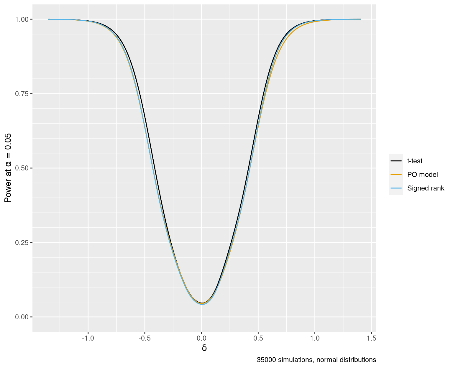
For our simulation model we use a situation that is ideal for the paired \(t\)-test and consider a sample size of \(n=25\) and hold \(\alpha=0.05\). We sample from a bivariate normal distribution where the correlation of the pair of random variables is 0.5, both variables have \(\sigma=1\), the first variable has mean 0 and the second mean \(\delta\). \(\delta\) is varied randomly to have a normal distribution with \(\sigma=0.4\) except that extra studies are simulated from exactly \(\delta=0\) so that we can accurately estimate type I assertion probability \(\alpha\).
For each of 35,000 simulated studies we compute p-values for the \(t\)-test, PO model with cluster sandwich correction, and the Wilcoxon signed-rank test, which is known to be \(\frac{3}{\pi} \approx 0.95\) as efficient as the \(t\) test in these ideal conditions.
The power of the PO test blocking on subject was attempted to be simulated but the model fit usually would not converge.
runParallel and runifChanged are in the Hmisc package and are discussed in R Workflow. runifChanged only runs the simulation if code or inputs changed, and runParallel breaks up the simulations to run simultaneously on as many CPU cores as available, less one.
To estimate power, binary logistic regression with a restricted cubic spline in \(\delta\) with 8 default knots is used. This is more precise than creating \(\delta\) intervals and computing simple proportions.
rms requires the datadist result to be stored in the global environment
Spearman ρ for p-values
       pt   ppo   psr
pt  1.000 0.954 0.975
ppo 0.954 1.000 0.943
psr 0.975 0.943 1.000
Under a nominal \(\alpha=0.05\) the true \(\alpha\) for the paired \(t\)-test is 0.05 and was estimated to be 0.048 from the 4400 simulations under the null \(\delta=0\). \(\alpha\) for the PO test was estimated to be 0.046 and for the signed-rank test was 0.043. Spearman rank correlations between the p-values for the two methods are given above.
Bivariate Log-normal Distribution
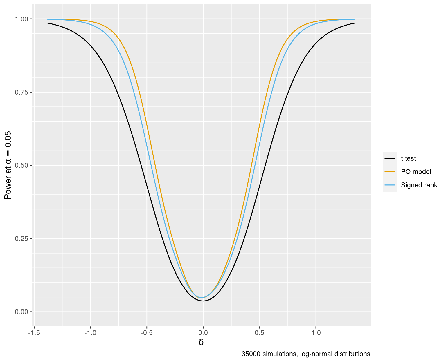
Now consider a situation where to satisfy the assumptions of the paired \(t\)-test and the Wilcoxon signed-rank test one would need to log the values before computing differences. Like the rank difference test, the PO model test is invariant to order-preserving transformations. Let’s simulate the operating characteristics for the same setup as before but taking anti-logs of the paired values. The three tests are not informed of the need to take logs to make the paired differences symmetric with constant variance.
Spearman ρ for p-values
       pt   ppo   psr
pt  1.000 0.714 0.823
ppo 0.714 1.000 0.887
psr 0.823 0.887 1.000
Code
w$graph
Note the lower correlations between p-values, especially for the \(t\)-test vs. the others. There is a significant loss of power for the \(t\)-test because of the large amount of skewness in the data. The signed-rank test lost a little power, and the PO model performs the same as under the ideal normality situation.
Under a nominal \(\alpha=0.05\) the true \(\alpha\) for the paired \(t\)-test was estimated to be 0.041 from the 4400 simulations under the null \(\delta=0\). \(\alpha\) for the PO test was estimated to be 0.05 and for the signed-rank test was 0.051.
Summary
Under an optimal parametric test setting the frequentist operating characteristics of the three tests are indistinguishable. The cluster sandwich correction for the standard error of the treatment effect estimated by the PO model (a log odds ratio) is solid.
The PO model with a cluster correlation correction preserves \(\alpha\) in the setting studied, and has only the slightest reduction in power when compared to the parametric test when all of the parametric test’s assumptions are satisfied. This reduction is similar to Wilcoxon signed-rank test’s performance, but the ordinal regression approach does not assume a correct transformation for the measurements has been specified, as shown with its preservation of power in the non-normal simulation example. The regression approach also generalizes to longitudinal data (not just two periods as studied here) and to include baseline covariate adjustment, unlike the signed-rank and rank difference tests. The power of the semiparametric modeling approach exceeds that of the paired \(t\)-test when the latter’s assumptions are violated.
Even though the cluster sandwich estimator performed perfectly in the situation studied, a full likelihood approach may be preferred. This is best done using random intercepts for subjects in a mixed-effects ordinal model using Bayesian posterior distribution Monte Carlo sampling, as current frequentist methods for this setting do not perform well due to the approximations used for marginalizing high-dimensional random effects when the sample size is not huge.
Ordinal models have an advantage over nonparametric tests such as the signed-rank test: post-regression-parameter-estimation one can compute a wide variety of model-based estimated effects including odds ratios, per-treatment exceedance probabilities, means, differences in means, ratios of means, differences in medians, ratios of medians, and other quantiles. Details are provided here. The bootstrap can be used to obtain approximate confidence intervals for these derived quantities, or Bayesian posterior sampling can be used to obtain exact uncertainty intervals.
Another advantage of modeling is that better utilization can be made of partial information. For example, if some subjects had only one of the two measurements of the pair, those subjects still contribute information to the PO model fit with robust sandwich estimator.
Computing Environment
Code
markupSpecs$html$session()
 R version 4.3.1 (2023-06-16)
 Platform: x86_64-pc-linux-gnu (64-bit)
 Running under: Pop!_OS 22.04 LTS

 Matrix products: default
 BLAS:   /usr/lib/x86_64-linux-gnu/blas/libblas.so.3.10.0
 LAPACK: /usr/lib/x86_64-linux-gnu/lapack/liblapack.so.3.10.0

 attached base packages:
 [1] stats     graphics  grDevices utils     datasets  methods   base

 other attached packages:
 [1] ggplot2_3.4.3 rms_6.7-1     Hmisc_5.1-1
To cite R in publications use:
R Core Team (2023).
R: A Language and Environment for Statistical Computing.
R Foundation for Statistical Computing, Vienna, Austria.
https://www.R-project.org/.
---title: Ordinal Models for Paired Dataauthor: - name: Frank Harrell affiliation: Department of Biostatistics<br>Vanderbilt University School of Medicine url: https://hbiostat.orgdate: 2023-08-16categories: [2023, ordinal, hypothesis-testing, inference, regression]description: "This article briefly discusses why the rank difference test is better than the Wilcoxon signed-rank test for paired data, then shows how to generalize the rank difference test using the proportional odds ordinal logistic semiparametric regression model. To make the regression model work for non-independent (paired) measurements, the robust cluster sandwich covariance estimator is used for the log odds ratio. Power and type I assertion $\\alpha$ probabilities are compared with the paired $t$-test for $n=25$. The ordinal model yields $\\alpha=0.05$ under the null and has power that is virtually as good as the optimum paired $t$-test. For non-normal data the ordinal model power exceeds that of the parametric test."---```{r setup, include=FALSE}require(rms)require(ggplot2)knitrSet(lang='quarto')```# BackgroundInstead of continually teaching special case statistical tests, I prefer to teach general models that include tests as special cases. For the usual cross-sectional or longitudinal layouts this is quite standard. But for paired data, practitioners are not so used to seeing a model-based approach.For paired data from a bivariate normal distribution, or for within-pair differences having a normal distribution, the paired $t$-test is a standard procedure. [BBR](https://hbiostat.org/bbr/nonpar.html#sec-nonpar-pairmodel) discussed how easy it is to get the same answer as the paired $t$-test using either an ordinary linear model blocking on subject or using a mixed effects model with random intercepts for subjects.[Surprisingly, the point estimate and standard error of the effect estimate are identical under the fixed effects and random effects models.]{.aside} That BBR section also shows some examples using ordinal regression. Note that ordinal regression works as well for [continuous response variables](https://hbiostat.org/rmsc/cony.html) as it does for discrete ordinal and binary ones.# Rank Difference TestFor unpaired data, the Wilcoxon-Mann-Whitney two-sample rank-sum test has the property that the p-value does not change if the response variable Y is monotonically transformed (logged, etc.). That is also true of the generalization of the Wilcoxon test, the proportional odds (PO) ordinal logistic semiparametric regression model. For paired data, the Wilcoxon signed-rank test does not share this transformation invariance property. One must know how to transform Y before computing the within-pair differences. Different transformations will result in different rankings of the differences. For this reason, [Kornbrot](https://doi.org/10.1111/j.2044-8317.1990.tb00939.x) introduced the rank difference test, which is transformation invariant. The rank difference test involves ranking $2n$ values for $n$ subjects each contributing a pair of correlated values. The pairing is accounted for when computing p-values.To generalize the rank difference test, the same data layout can be applied to an ordinary PO model. Unfortunately, the linear model formulation of blocking on subjects and testing a binary treatment variable does not work because of the large number of parameters (subjects), resulting in great instability and failure to preserve $\alpha$ in a regular PO model. A random effects frequentist PO model was also tried in BBR, but the standard error of the treatment effect was far too low. A Bayesian random effects PO model seemed to work well.# Ordinal Model for Paired DataIt would be nice if there were a PO model approach to paired data that did not require the use of random effects for subjects. [Noah Greifer](https://ngreifer.github.io) suggested the use of the [robust cluster sandwich covariance correction](https://stats.stackexchange.com/questions/622981). The cluster sandwich estimator corrects standard errors for intra-class correlation and works especially well with a large number of small clusters. Here we have two observations per subject, barring any missing data. The `rms` package's `robcov` function replaces the variance-covariance matrix of estimated regression coefficients with the cluster sandwich estimates. See also the [sandwich package](https://cran.r-project.org/web/packages/sandwich).# Small Simulation Study## Bivariate Normal DistributionFor our simulation model we use a situation that is ideal for the paired $t$-test and consider a sample size of $n=25$ and hold $\alpha=0.05$. We sample from a bivariate normal distribution where the correlation of the pair of random variables is 0.5, both variables have $\sigma=1$, the first variable has mean 0 and the second mean $\delta$. $\delta$ is varied randomly to have a normal distribution with $\sigma=0.4$ except that extra studies are simulated from exactly $\delta=0$ so that we can accurately estimate type I assertion probability $\alpha$.For each of 35,000 simulated studies we compute p-values for the $t$-test, PO model with cluster sandwich correction, and the Wilcoxon signed-rank test, which is known to be $\frac{3}{\pi} \approx 0.95$ as efficient as the $t$ test in these ideal conditions. [The power of the PO test blocking on subject was attempted to be simulated but the model fit usually would not converge.]{.aside}```{r sim1}sim <-function(nsim, nnull=0, n=25, rho=0.5, trans=function(x) x,check=FALSE, showprogress, core) { delta <- pt <- ppo <- psr <-numeric(nsim) id <-factor(1: n) id <-c(id, id) x <-c(rep(0, n), rep(1, n)) z <-matrix(NA, nrow=nsim, ncol=6,dimnames=list(NULL, .q(delta, mean1, mean2, sd1, sd2, r)))for(i in1: nsim) {showprogress(i, nsim, core) delta[i] <-if(i <= nnull) 0.elsernorm(1, 0, 0.4) y1 <-rnorm(n) y2 <-rnorm(n, delta[i] + rho * y1, sqrt(1- rho^2)) #<1> z[i, ] <-c(delta[i], mean(y1), mean(y2), sd(y1), sd(y2), cor(y1, y2)) y1 <-trans(y1) y2 <-trans(y2) pt[i] <-t.test(y1, y2, paired=TRUE)$p.value y <-c(y1, y2) f <-orm(y ~ x, x=TRUE, y=TRUE, maxit=200) g <-robcov(f, id) ppo[i] <-anova(g)['x', 'P'] psr[i] <-wilcox.test(y1, y2, paired=TRUE)$p.value }if(check) {plsmo(z[, 'delta'], z[, 'mean2'])plsmo(z[, 'delta'], z[, 'mean2'] - z[, 'mean1'])print(apply(z, 2, mean)) }data.frame(delta, pt, ppo, psr)}run1 <-function(reps, showprogress, core)sim(nsim=reps, nnull=400, showprogress=showprogress, core=core)g <-function() runParallel(run1, reps=35000, seed=13) #<2>sim1 <-runifChanged(g, run1, sim)```1. See [here](https://blog.revolutionanalytics.com/2016/08/simulating-form-the-bivariate-normal-distribution-in-r-1.html)2. `runParallel` and `runifChanged` are in the `Hmisc` package and are discussed in [R Workflow](https://hbiostat.org/rflow). `runifChanged` only runs the simulation if code or inputs changed, and `runParallel` breaks up the simulations to run simultaneously on as many CPU cores as available, less one.To estimate power, binary logistic regression with a restricted cubic spline in $\delta$ with 8 default knots is used. This is more precise than creating $\delta$ intervals and computing simple proportions.```{r sum}#| fig.width: 8#| fig.height: 6.5sumz <-function(s, desc='') { s <-as.data.frame(s) dd <<-datadist(s); options(datadist='dd') #<1> null <- s$delta ==0. alpha <-with(s, list(t =mean(pt[null] <0.05),po =mean(ppo[null] <0.05),sr =mean(psr[null] <0.05))) alpha <-lapply(alpha, round, digits=3) rho =with(s, round(rcorr(cbind(pt, ppo, psr), type='spearman')$r, 3))cat('Spearman ρ for p-values\n')print(rho) mx <-30; tol=1e-10 f <-lrm(pt <0.05~rcs(delta, 8), data=s, maxit=mx, tol=tol) p1 <-Predict(f, delta, fun=plogis, conf.int=FALSE) g <-lrm(ppo <0.05~rcs(delta, 8), data=s, maxit=mx, tol=tol) p2 <-Predict(g, delta, fun=plogis, conf.int=FALSE) h <-lrm(psr <0.05~rcs(delta, 8), data=s, maxit=mx, tol=tol) p3 <-Predict(h, delta, fun=plogis, conf.int=FALSE) p <-rbind('t-test'=p1, 'PO model'=p2, 'Signed rank'=p3) graph <-ggplot(p, aes(delta, yhat, color=.set.)) +geom_line() +ylab(expression(paste('Power at ', alpha==0.05))) +guides(color=guide_legend(title='')) +labs(caption=paste0(nrow(s), ' simulations', if(desc !='') paste0(', ', desc))) +scale_y_continuous(minor_breaks=seq(0, 1, by=0.05))list(alpha=alpha, graph=graph)}w <-sumz(sim1, 'normal distributions')w$graph```1. `rms` requires the `datadist` result to be stored in the global environmentUnder a nominal $\alpha=0.05$ the true $\alpha$ for the paired $t$-test is 0.05 and was estimated to be `r w$alpha$t` from the `r sum(sim1$delta == 0.)` simulations under the null $\delta=0$. $\alpha$ for the PO test was estimated to be `r w$alpha$po` and for the signed-rank test was `r w$alpha$sr`. Spearman rank correlations between the `r nrow(sim1)` p-values for the two methods are given above.## Bivariate Log-normal DistributionNow consider a situation where to satisfy the assumptions of the paired $t$-test and the Wilcoxon signed-rank test one would need to log the values before computing differences. Like the rank difference test, the PO model test is invariant to order-preserving transformations. Let's simulate the operating characteristics for the same setup as before but taking anti-logs of the paired values. The three tests are not informed of the need to take logs to make the paired differences symmetric with constant variance.```{r sim2}#| fig.width: 8#| fig.height: 6.5run1 <-function(reps, showprogress, core)sim(nsim=reps, nnull=400, trans=exp, showprogress=showprogress, core=core)g <-function() runParallel(run1, reps=35000, seed=4)sim2 <-runifChanged(g, run1, sim)w <-sumz(sim2, 'log-normal distributions')w$graph```Note the lower correlations between p-values, especially for the $t$-test vs. the others.There is a significant loss of power for the $t$-test because of the large amount of skewness in the data. The signed-rank test lost a little power, and the PO model performs the same as under the ideal normality situation.Under a nominal $\alpha=0.05$ the true $\alpha$ for the paired $t$-test was estimated to be `r w$alpha$t` from the `r sum(sim2$delta == 0.)` simulations under the null $\delta=0$. $\alpha$ for the PO test was estimated to be `r w$alpha$po` and for the signed-rank test was `r w$alpha$sr`. # SummaryUnder an optimal parametric test setting the frequentist operating characteristics of the three tests are indistinguishable. The cluster sandwich correction for the standard error of the treatment effect estimated by the PO model (a log odds ratio) is solid.The PO model with a cluster correlation correction preserves $\alpha$ in the setting studied, and has only the slightest reduction in power when compared to the parametric test when all of the parametric test's assumptions are satisfied. This reduction is similar to Wilcoxon signed-rank test's performance, but the ordinal regression approach does not assume a correct transformation for the measurements has been specified, as shown with its preservation of power in the non-normal simulation example. The regression approach also generalizes to longitudinal data (not just two periods as studied here) and to include baseline covariate adjustment, unlike the signed-rank and rank difference tests. The power of the semiparametric modeling approach exceeds that of the paired $t$-test when the latter's assumptions are violated.Even though the cluster sandwich estimator performed perfectly in the situation studied, a full likelihood approach may be preferred. This is best done using random intercepts for subjects in a mixed-effects ordinal model using Bayesian posterior distribution Monte Carlo sampling, as current frequentist methods for this setting do not perform well due to the approximations used for marginalizing high-dimensional random effects when the sample size is not huge.Ordinal models have an advantage over nonparametric tests such as the signed-rank test: post-regression-parameter-estimation one can compute a wide variety of model-based estimated effects including odds ratios, per-treatment exceedance probabilities, means, differences in means, ratios of means, differences in medians, ratios of medians, and other quantiles. Details are provided [here](https://hbiostat.org/rmsc/cony.html). The bootstrap can be used to obtain approximate confidence intervals for these derived quantities, or Bayesian posterior sampling can be used to obtain exact uncertainty intervals.Another advantage of modeling is that better utilization can be made of partial information. For example, if some subjects had only one of the two measurements of the pair, those subjects still contribute information to the PO model fit with robust sandwich estimator.# Computing Environment```{r results='asis'}markupSpecs$html$session()```