Proportional Odds Model Power Calculations for Ordinal and Mixed Ordinal/Continuous Outcomes

inference

hypothesis-testing

regression

ordinal

change-scores

design

endpoints

medicine

sample-size

2024

This article has detailed examples with complete R code for computing frequentist power for ordinal, continuous, and mixed ordinal/continuous outcomes in two-group comparisons with equal sample sizes. Mixed outcomes allow one to easily handle clinical event overrides of continuous response variables. The proportional odds model is used throughout, and care is taken to convert odds ratios to differences in medians or means to aid in understanding effect sizes. Since the Wilcoxon test is a special case of the proportional odds model, the examples also show how to tailor sample size calculations to the Wilcoxon test, at least when there are no covariates.

Author

Affiliation

Frank Harrell

Department of Biostatistics
Vanderbilt University School of Medicine

Published

April 22, 2024

Modified

April 22, 2024

Background

A binary endpoint in a clinical trial is a minimum-information endpoint that yields the lowest power for treatment comparisons. A time-to-event outcome, when only a minority of subjects suffer the event, has little power gain over a pure binary endpoint, since its power comes from the number of events (number of uncensored observations). The highest power endpoint would be from a continuous variable that is measured precisely and reflects the clinical outcome situation. An ordinal outcome with, say, five or more well-populated levels yields power that can approach that of a truly continuous outcome. When the original binary outcome represents the union of several clinical endpoints, the analysis treats all endpoints as equally important. An ordinal outcome variable, even if it has only a few levels, breaks the ties and improves power. When there are clinical responses that are ordinal or continuous and one is willing to assume that any clinical event overrides any level of such a scale, one can easily construct an ordinal scale that incorporates both clinical events and the scale. A great advantage of this approach, besides improved power, is that it gives one a place to record bad clinical events such as death, without the need for using a complex statistical analysis that has to deal with such questions as “what would have happened had the patient not died” or “how do I handle missing data when the patient died before the ordinal/continuous was measured?”.

Continuous and ordinal scales can be compared between treatment groups using the Wilcoxon-Mann-Whitney two-sample test. This does not allow for adjustment of covariates, nor does it properly handle a large number of ties in the patient responses. The proportional odds (PO) ordinal logistic regression model is a generalization of the Wilcoxon test, and it handles arbitrarily heavy ties. Since the Wilcoxon test assumes within-group homogeneity of outcome tendencies, the Wilcoxon test makes more assumptions than the PO model. We will use the PO model in what follows. For now we consider the oversimplified situation in which a patient has recorded the worst category outcome that occurred within 12m of randomization. For the actual clinical trial analysis we might use a longitudinal Markov state transition model in which the ordinal outcome scale is assessed weekly until the patient dies or follow-up ends. This approach counts multiple hospitalizations as having more weight than a single hospitalization. Since the power calculations below use only one overall measurement per patient, it represents a lower bound on the power that will actually be obtained. The power formula used here is due to Whitehead¹ using the R² Hmisc package function popower or by simulation using the simRegOrd function³.

The PO model handles treatment effects through odds ratios. Let the ordinal outcome be denoted by \(Y\) and one of its levels be \(y\). Consider the probability that \(Y \geq y\) for a patient on treatment A and for a patient on treatment B. The odds that \(Y \geq y\) for a treatment is the probability divided by one minus the probability. The B : A odds ratio for \(Y \geq y\) is some constant OR and by the PO assumption this OR is the same no matter which cutoff y is chosen. When the hard clinical events are at the high end of the ordinal scale and a patient oriented outcome scale is at the low end, the PO model assumes that the treatment effect (on the OR scale) for, say, death is the same as the OR for the outcome scale being worse than any given level or the patient dying. When the treatment has a different effect on nonfatal outcomes as for fatal ones, the overall OR represents a kind of weighted average over the various treatment effects. See this for an example where the treatment effect on death is allowed to differ from the effect on nonfatal outcomes when computing power.

Initially Considered Outcome Scale

Consider the Kansas City Cardiomyopathy Questionnaire of JA Spertus et al, which measures symptoms, social and physical limitations, and quality of life in heart failure patients. KCCQ ranges from 0 to 100 with 100 being the most desirable outcome. To account for clinical events, we extend the KCCQ scale with three clinical event overrides. Assume that KCCQ and event status are assessed one year post randomization.

Y	Meaning
103	Cardiovascular death
102	Non-cardiovascular death
101	Hospitalization for HF/Renal Disease
100	KCCQ=0
99	KCCQ=1
..	…
1	KCCQ=99
0	KCCQ=100

KCCQ is the 1 year KCCQ overall summary score. Non-CV death is placed after CV death because we wanted to give more weight to treatment effects on the latter, and we expect less effect on the former. For the actual analysis of trial data, KCCQ will have non-integer values and will be analyzed as a continuous variable, i.e., there will be one intercept in the PO model per distinct value of KCCQ, less one, plus three for clinical events.

A sample of KCCQ summary scores was provided by Vanderbilt cardiologist Brian Lindman, for which summary statistics are shown below along with a histogram.

Code

require(rms)
require(data.table)
require(ggplot2)
options(prType='html', grType='plotly')
d    <- csv.get('dd.csv')
d$id <- NULL
k <- d$kccq1
describe(d)

d Descriptives

d

6 Variables 373 Observations

age

n	missing	distinct	Info	Mean	Gmd	.05	.10	.25	.50	.75	.90	.95
373	0	43	0.998	81.64	8.849	65.6	70.0	78.0	83.0	87.0	90.0	92.0

lowest : 38 55 57 58 59 , highest: 93 94 95 97 100

sex

n	missing	distinct
373	0	2

 Value      Female   Male
 Frequency     169    204
 Proportion  0.453  0.547

scr0

n	missing	distinct	Info	Mean	Gmd	.05	.10	.25	.50	.75	.90	.95
372	1	140	1	1.286	0.6279	0.6755	0.7510	0.8900	1.1000	1.4500	1.7800	2.2425

lowest : 0.34 0.47 0.49 0.56 0.58 , highest: 4.9 5.37 6.6 7.76 10.11

kccq0

n	missing	distinct	Info	Mean	Gmd	.05	.10	.25	.50	.75	.90	.95
345	28	161	1	46.7	27.85	10.80	15.63	27.08	43.23	64.58	83.33	89.06

lowest : 0 2.08 3.13 4.17 5.21 , highest: 93.75 95.83 96.88 97.4 100

scr1

n	missing	distinct	Info	Mean	Gmd	.05	.10	.25	.50	.75	.90	.95
202	171	95	0.999	1.33	0.7002	0.690	0.750	0.900	1.155	1.487	1.879	2.400

lowest : 0.45 0.5 0.57 0.6 0.63 , highest: 3.2 3.7 5.3 6.1 11.7

kccq1

n	missing	distinct	Info	Mean	Gmd	.05	.10	.25	.50	.75	.90	.95
373	0	146	0.998	72.06	27.65	23.75	33.33	55.56	78.47	93.75	100.00	100.00

lowest : 0 2.08 8.85 10.42 11.46 , highest: 97.92 98.44 98.61 98.96 100

1y vs. Baseline KCCQ

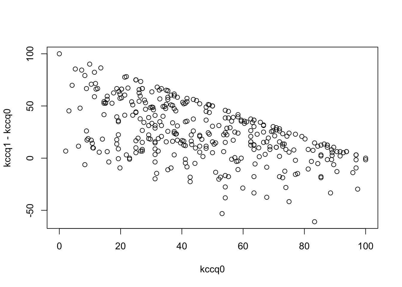
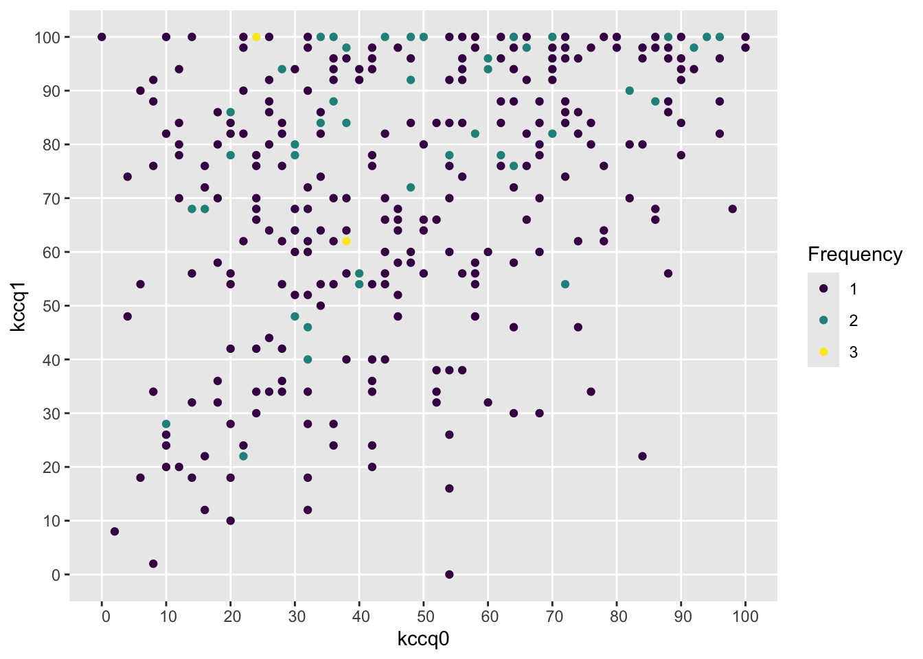
Severe problems, especially a ceiling effect, are seen in using change in KCCQ from baseline, and the slope is far less than 1.0. The first graph below should trend flat with equal variability going across.

Code

with(d, plot(kccq0, kccq1 - kccq0))

Code

with(d, ggfreqScatter(kccq0, kccq1))

Code

ggplot(d, aes(x=kccq0, y=kccq1)) + geom_point() + geom_smooth()

Code

with(d, spearman(kccq0, kccq1))

rho

0.3564163

Code

f <- ols(kccq1 ~ kccq0, data=d)
f

Linear Regression Model

ols(formula = kccq1 ~ kccq0, data = d)

Frequencies of Missing Values Due to Each Variable

kccq1 kccq0 
    0    28

	Model Likelihood Ratio Test	Discrimination Indexes
Obs 345	LR χ² 50.86	R² 0.137
σ 23.1606	d.f. 1	R²_adj 0.135
d.f. 343	Pr(>χ²) 0.0000	g 10.572

Residuals

    Min      1Q  Median      3Q     Max 
-73.724 -16.255   3.432  17.476  46.445

	β	S.E.	t	Pr(>\|t\|)
Intercept	53.5546	2.7063	19.79	<0.0001
kccq0	0.3796	0.0514	7.38	<0.0001

Code

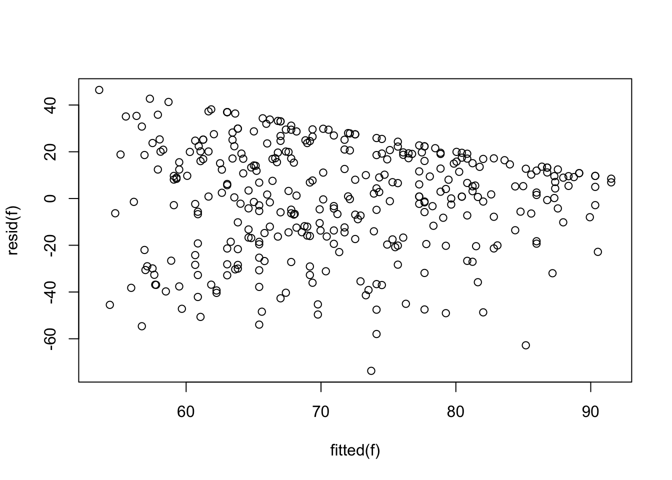
plot(fitted(f), resid(f))

Code

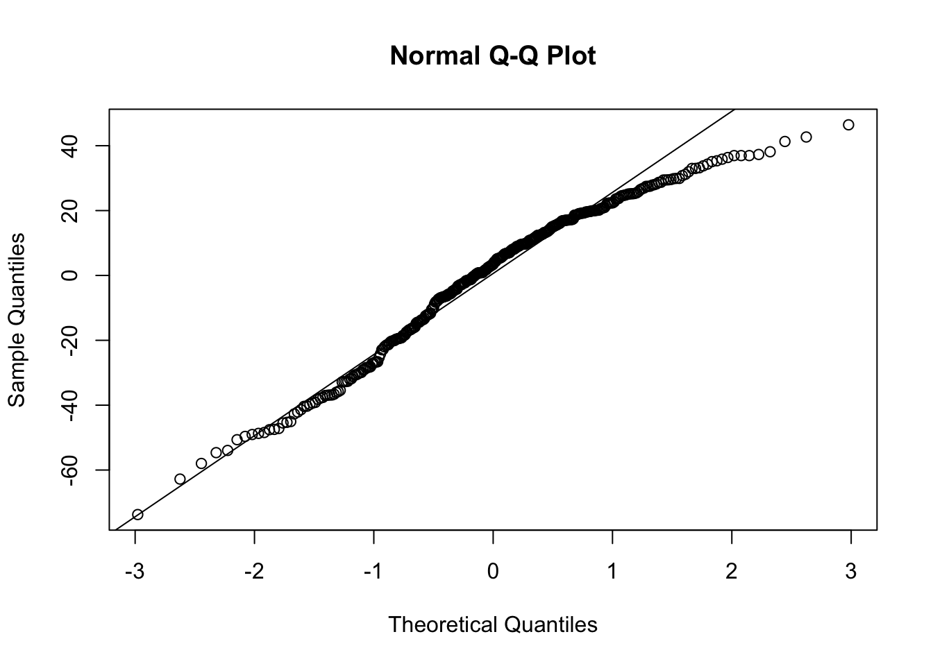
qqnorm(resid(f))
qqline(resid(f))

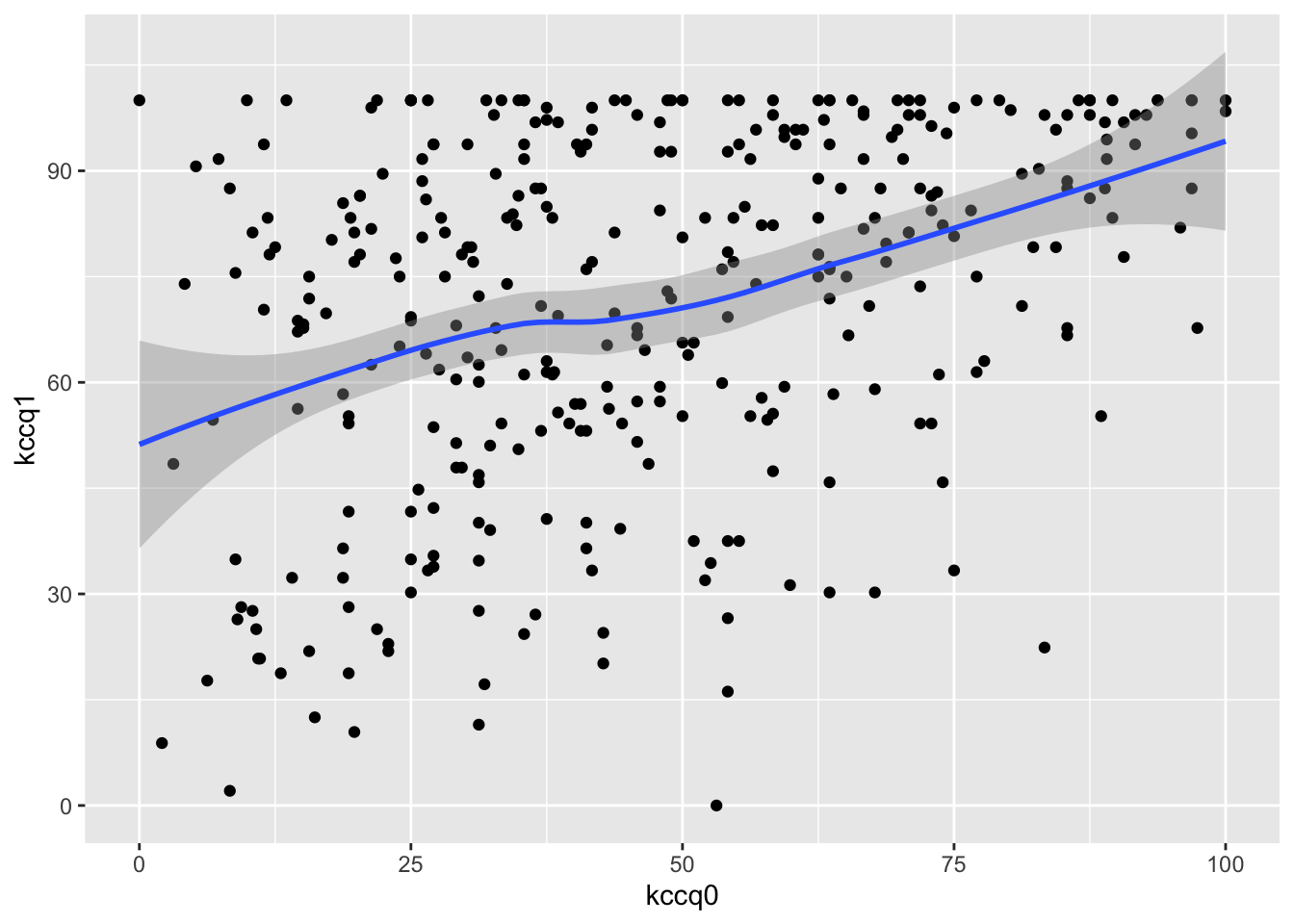
The last graph should be a straight line if normality holds, and the one before that should trend flat with constant variability as you look left to right. There is a very strong ceiling effect, and the slope of 1.0 on post vs. pre that is needed for a simple change score analysis is far from the estimated slope of 0.38.

Point of Reference: Power for Traditional Outcomes

KCCQ As a Continuous Variable

For comparison purposes, we compute the power of the 2-sample t-test for detecting a 5-unit difference in mean KCCQ using the standard deviation of the above KCCQ sample (SD = 24.9). The assumed sample size is n=300 (both groups combined).

Code

require(pwr)
pwr.t.test(n=300/2, d=5/sd(k), type='two.sample')


     Two-sample t test power calculation 

              n = 150
              d = 0.2011522
      sig.level = 0.05
          power = 0.4116635
    alternative = two.sided

NOTE: n is number in *each* group

Code

r1 <- function(x) round(x, 1)

Because KCCQ is not very normally distributed (e.g., has lots of ties at its ceiling value of 100), we also compute the power of the Wilcoxon/proportional odds model test. To do this we need to specify an odds ratio. We do this by applying a series of odds ratios and computing the difference in mean and median KCCQ score as compared to an odds ratio of 1. The mean and median of the provided KCCQ sample are 72.1 and 78.5, respectively. We consider 100 - KCCQ (because that is how the odds ratio will be applied later) although this may not matter.

Code

kp <- table(round(100 - k, 2)); kp <- kp / sum(kp)
kx <- as.numeric(names(kp))
# First check against original values by using an odds ratio of 1
w <- pomodm(kx, kp, odds.ratio=1)
w

    mean   median 
27.93547 21.44000

Code

ors <- seq(0.2, 1, length=200)
z <- data.table(or=ors)
u <- z[, as.list(w - pomodm(kx, kp, odds.ratio=or)), by=or]
m <- meltData(or ~ mean + median, data=u)   # is in Hmisc
ggplot(m, aes(x=or, y=value, color=variable)) + geom_line() +
  geom_vline(xintercept=0.685, alpha=0.3) +
  guides(color=guide_legend(title='')) +
  xlab('Odds Ratio') + ylab('Difference Between Groups')

So let’s compute the Wilcoxon test power for KCCQ alone at an odds ratio of 0.685 (vertical gray scale line in previous plot).

Code

popower(kp, odds.ratio=0.685, 300)

Power: 0.47 
Efficiency of design compared with continuous response: 0.998 
Approximate standard error of log odds ratio: 0.2009

This power is a bit higher than the power of the t-test which (problematically) assumed normality. Non-symmetry of the data distribution probably makes the standard deviation not be a good measure of dispersion, and this damages performances of the t-test.

Binary Outcome

For comparison of binary outcomes, consider these endpoint scenarios.

Code

n <- c('CV Death', 'Non-CV Death', 'Hosp for HF/Renal', 'No Event')
phigh <- c(0.078, 0.052, 0.10) * 2 / 3; phigh <- c(phigh, 1 - sum(phigh))
plow  <- c(0.054, 0.036, 0.06) * 2 / 3; plow  <- c(plow,  1 - sum(plow))
x <- rbind(phigh, plow)
rownames(x) <- c('High Risk', 'Low Risk')
colnames(x) <- n
x

          CV Death Non-CV Death Hosp for HF/Renal  No Event
High Risk    0.052   0.03466667        0.06666667 0.8466667
Low Risk     0.036   0.02400000        0.04000000 0.9000000

For a simple power calculation let’s use the high-risk scenario and combine the three endpoints, for an overall incidence of 0.23. The power to detect a treatment effect than is an odds ratio of 0.8 for a total sample size of 300 is:

Code

bpower(0.23, odds.ratio=0.8, n=300)

    Power 
0.1232294

Code

p2 <- plogis(qlogis(0.23) + log(0.8))

The odds ratio of 0.8 corresponds to reducing the risk of 0.23 to 0.193. An odds ratio of 0.7 would increase the power to:

Code

bpower(0.23, odds.ratio=0.7, n=300)

   Power 
0.233493

Code

p2 <- plogis(qlogis(0.23) + log(0.7))

This is the power to detect a reduction from 0.23 to 0.173.

Mixed Continuous / Clinical Event Endpoint

We tabulate the frequency distribution of the above KCCQ sample and assume two different scenarios for the clinical endpoint overrides. For both the high-risk and low-risk scenarios, we distribute the proportion of non-events across the same distribution of KCCQs. KCCQ is reflected about 100 to make smaller values = better outcomes.

Code

# Assign the sum of kp to the prob. of "no event"
# Function to put events together with KCCQ distribution for an overall ordinal scale
f <- function(p) {
  no.event <- p[4]
  n <- c(n[1 : 3], names(kp))
  # Make kp sum to prob of no event instead of 1.0
  kp <- kp * p[4]
  pr <- c(kp, p[3 : 1])
  names(pr) <- c(names(kp), 101, 102, 103)
  pr
}
yhigh <- f(phigh)
ylow  <- f(plow)
P     <- cbind(high=yhigh, low=ylow)
xp    <- as.numeric(names(yhigh))

a <- pomodm(xp, yhigh, odds.ratio=1)
b <- pomodm(xp, ylow,  odds.ratio=1)
z <- cbind(
         'Y Mean'       = c(a[1], b[1]),                
         'Y Median'     = c(a[2], b[2]),
           'KCCQ+ Mean'   = 100 - c(a[1], b[1]),
           'KCCQ+ Median' = 100 - c(a[2], b[2]),
             'KCCQ Mean'    = rep(mean(k), 2),
             'KCCQ Median'  = rep(median(k), 2))
rownames(z) <- c('high', 'low')
z

       Y Mean Y Median KCCQ+ Mean KCCQ+ Median KCCQ Mean KCCQ Median
high 39.27736 28.97878   60.72264     71.02122  72.06453       78.47
low  35.33792 25.15889   64.66208     74.84111  72.06453       78.47

Power Calculations

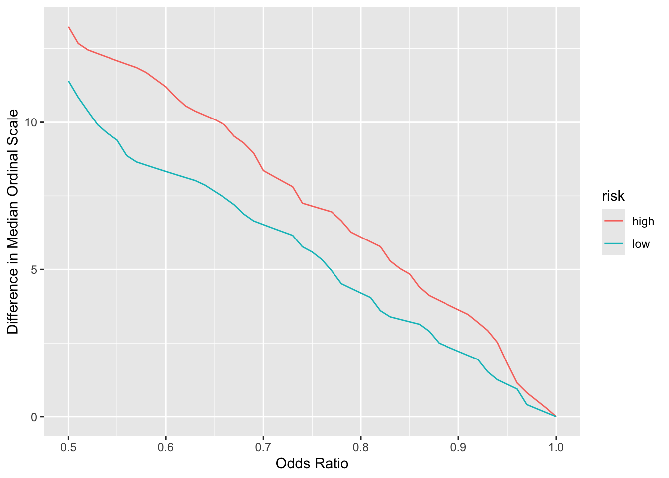
Compute power for the unadjusted two-sample proportional odds model treatment comparison (Wilcoxon test but handles ties better). For interpreting results on the original scale, concentrate on the median as the mean is dependent on the numeric codes assigned to clinical events. The median only relies on the ordering, as long as clinical events have incidence \(< \frac{1}{2}\).

Code

# Compute difference in median ordinal values as a function of or
y <- expand.grid(or   = seq(0.5, 1, by=0.01),
                 risk = c('high', 'low'))
medsor1 <- z[, 'Y Median']
setDT(y)
u <- y[, as.list(pomodm(xp, P[, risk], odds.ratio=or)), by=.(or, risk)]
u[, dmed := medsor1[risk] - median, by=.(or, risk)]

ggplot(u, aes(x=or, y=dmed, group=risk, color=risk)) + geom_line() +
  xlab('Odds Ratio') + ylab('Difference in Median Ordinal Scale')

Code

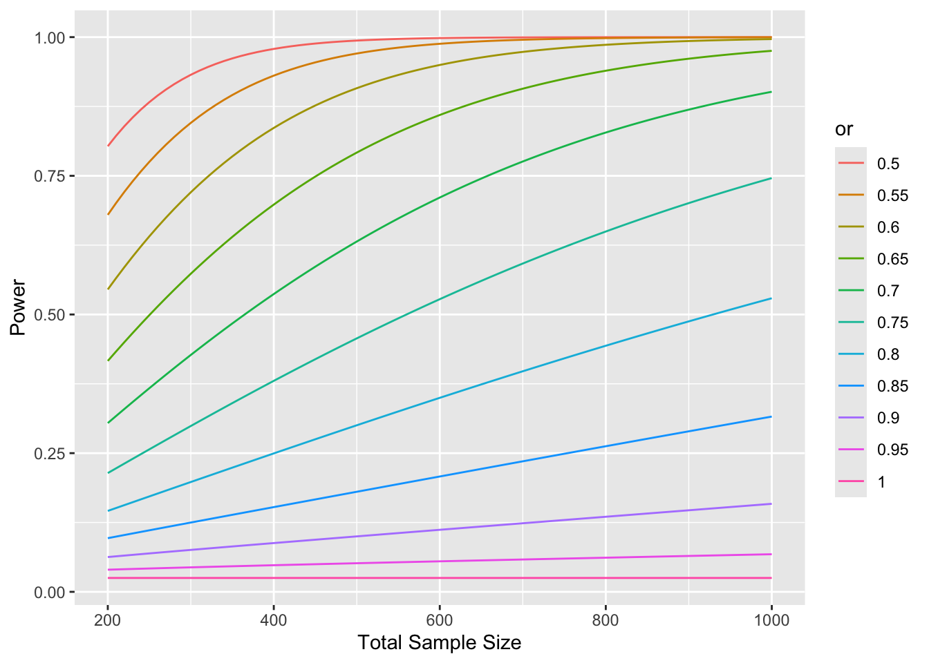
x <- expand.grid(n    = seq(200, 1000, by=10),
                 or   = seq(0.5, 1, by=0.05),
                 risk = c('high', 'low'))
setDT(x)
u <- x[, .(power = popower(P[, risk], odds.ratio=or, n=n)$power),
           by=.(n, or, risk)]
pdif <- u[risk == 'high', power] - u[risk == 'low', power]
mpdif <- max(abs(pdif))
cat('Maximum difference in power for low vs. high risk:', mpdif, '\n')

Maximum difference in power for low vs. high risk: 4.495558e-05

Code

u[, or := factor(or)]
ggplot(u[risk == 'low'],
       aes(x=n, y=power, group=or, color=or)) + geom_line() + 
  xlab('Total Sample Size') + ylab('Power')

BNP as an Outcome

Dr. Lindman provided information about baseline and 1y BNP levels.

Code

b <- csv.get('bnp.csv', lowernames=TRUE)
b <- subset(b, select=c(1, 2, 3, 11, 12))
names(b) <- Cs(id, type0, bnp0, type1, bnp1)
b <- subset(b, type0 == 'BNP' & type1 == 'BNP')

The relationship between baseline and 1y BNP is not linear (and the average slope is far from 1.0), so it is impossible to find a transformation (e.g., log) that will result in a valid change score for BNP. This is demonstrated below using the log transformation.

Code

dd <- datadist(b); options(datadist='dd')
f <- ols(log(bnp1) ~ rcs(log(bnp0), 5), data=b, x=TRUE)
f

Linear Regression Model

ols(formula = log(bnp1) ~ rcs(log(bnp0), 5), data = b, x = TRUE)

	Model Likelihood Ratio Test	Discrimination Indexes
Obs 181	LR χ² 125.73	R² 0.501
σ 0.6852	d.f. 4	R²_adj 0.489
d.f. 176	Pr(>χ²) 0.0000	g 0.723

Residuals

     Min       1Q   Median       3Q      Max 
-1.64421 -0.50473  0.03422  0.42261  1.72760

	β	S.E.	t	Pr(>\|t\|)
Intercept	0.3206	0.7565	0.42	0.6722
bnp0	0.9250	0.1764	5.24	<0.0001
bnp0'	-0.6749	0.8616	-0.78	0.4345
bnp0''	3.5123	4.8454	0.72	0.4695
bnp0'''	-7.8663	7.7603	-1.01	0.3121

Code

anova(f)

Analysis of Variance for `log(bnp1)`
	d.f.	Partial SS	MS	F	P
bnp0	4	82.889531	20.7223827	44.13	<0.0001
Nonlinear	3	8.816436	2.9388121	6.26	0.0005
REGRESSION	4	82.889531	20.7223827	44.13	<0.0001
ERROR	176	82.638057	0.4695344

Code

plotp(Predict(f, fun=exp), ylab='BNP at 1y')

Code

sigma <- f$stats['Sigma']

For the log model the residual standard deviation is 0.6852258. The SD of log BNP1 is 0.9589566 and the SD of the log ratio to baseline is 0.8260917. The smaller residual SD (which indicates a much better fit than a change score) will be the basis for the next power calculation below.

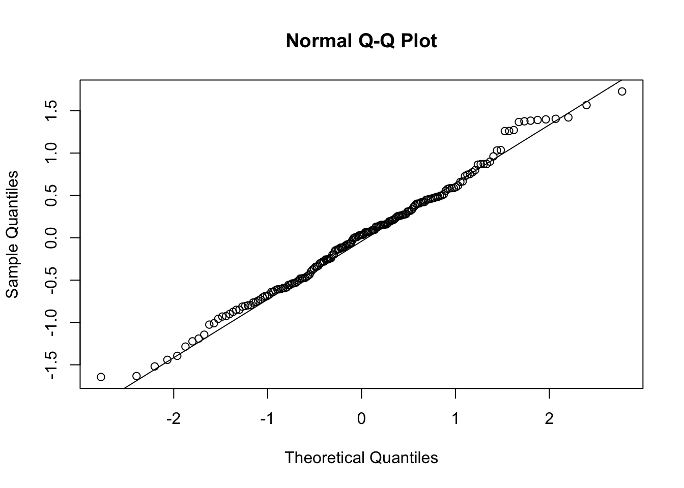
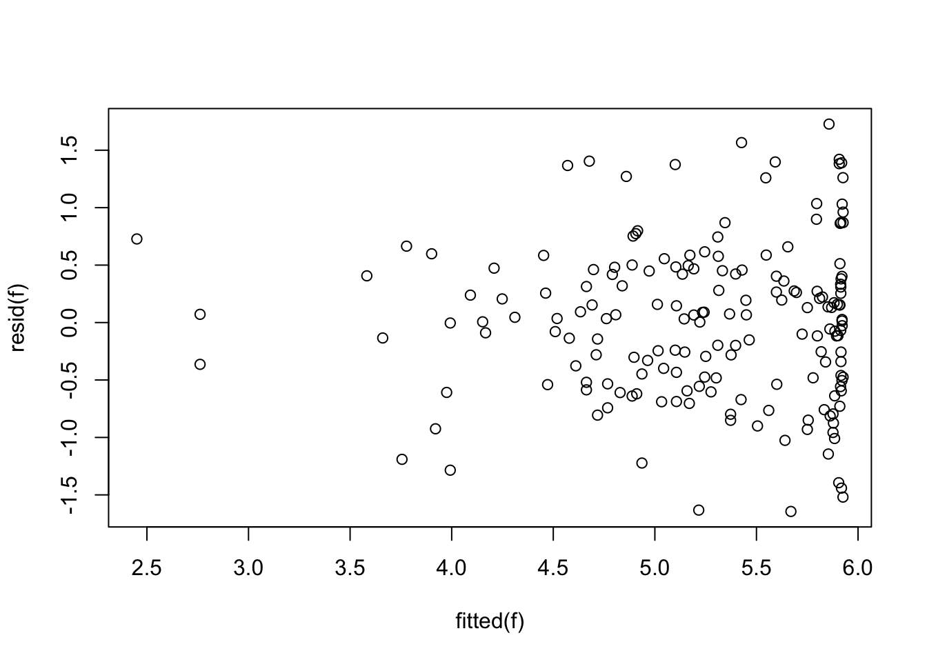
Next we check to see that the nonlinear model in baseline BNP satisfies the usual normality and equal variance assumptions.

Code

qqnorm(resid(f))
qqline(resid(f))

Code

plot(fitted(f), resid(f))

The assumptions are largely satisfied.

Power

Power of Classical ANCOVA on BNP alone

The first approximation of power is for comparing BNP at one year between treatment groups, ignoring clinical events, uses analysis of covariance (ANCOVA) adjusting for a nonlinear function of baseline BNP using a restricted cubic spline function with 5 knots (as used above). Power is calculated by inserting the residual SD above into the power function for the ordinary two-sample t-test. Because the ANCOVA model is based on log BNP, effects are stated as fold change. A total sample size of 300 is assumed.

Code

fc <- Power <- seq(.6, 1, length=200)
for(i in 1 : length(fc))
  Power[i] <- pwr.t.test(n=300/2, d=log(fc[i]) / sigma,
                                                type='two.sample')$power
# plot(fc, Power, xlab='Fold Change to Detect', type='l',
#      main='Power of 2-sample ANCOVA Test for BNP')
# abline(h=c(0.8, 0.9), col=gray(.8))
# abline(v=seq(0.6, 0.9, by=0.05), col=gray(.8))
require(plotly)
p <- add_lines(plot_ly(), x = ~ fc, y = ~ Power)
layout(p, xaxis=list(title='Fold Change to Detect'))

The actual analysis will be based on a proportional odds model with high-level category overrides for clinical events (see the next section). If the treatment has the same effect on clinical events as it does for BNP, and the clinical events are not too frequent, the power will be very similar to that depicted in the previous graph.

Power of Covariate-Adjusted Proportional Odds Model

Power of a covariate-adjusted proportional odds two-sample test must be estimated using simulation, even when there are no clinical endpoint overrides. Simulation will be done with the R Hmisc package simRegOrd function. This is done by simulating two normally-distributed random variables with equal variance, simulating ordinal clinical endpoints (including “no endpoint”), and for subjects for whom “no endpoint” was not the outcome, the continuous BNP values are overridden by the ordinal clinical values. Besides the sample size, type I assertion probability \(\alpha\), covariate distribution, and covariate effect, there are two parameters to specify for the power where there are clinical overrides: the odds ratio for the clinical endpoints and the difference in means. Here the latter is on the log BNP scale, so it represents log ratios. The odds ratio is left at 0.75 throughout, and the log BNP effect sizes are varied so that the following fold changes are used: 0.75, 0.8, 0.85, 0.9, 1.0.

The baseline BNP distribution is assumed to be the same as that in the pilot study. Baseline BNP values were generated by sampling with replacement from that study.

Note that the simulation is done so that clinical endpoints and BNP values are generated independently. In reality, these endpoints are more likely to be positively correlated.

Code

fc <- c(0.75, 0.8, 0.85, 0.9, 1.0)
# n  <- c(300, 326, 350, 376, 400)
n  <- c(250, 276, 300, 326, 350)
ev <- c('CV Death', 'Non-CV Death', 'Hosp for HF/Renal', 'Worsening HF',
        'No Event')
phigh <- c(0.078, 0.052, 0.10, 0.08) * 2 / 3;  phigh <- c(phigh, 1 - sum(phigh))
plow  <- c(0.054, 0.036, 0.06, 0.04) * 2 / 3;  plow  <- c(plow,  1 - sum(plow))
p <- rbind('High Risk'=rev(phigh), 'Low Risk'=rev(plow))
colnames(p) <- rev(ev)
p

           No Event Worsening HF Hosp for HF/Renal Non-CV Death CV Death
High Risk 0.7933333   0.05333333        0.06666667   0.03466667    0.052
Low Risk  0.8733333   0.02666667        0.04000000   0.02400000    0.036

Code

if(file.exists('powerOrd.rds')) z <- readRDS('powerOrd.rds') else {
z <- array(NA, dim=c(2, length(fc), length(n)),
           dimnames=list(rownames(p), as.character(fc), as.character(n)))
set.seed(4)
b0 <- b$bnp0[! is.na(b$bnp0)]
i  <- 0
for(nn in n) {
  j <- sample(1 : length(b0), nn, replace=nn > length(b0))
  x <- b0[j]
  X <- f$x[j, ]
  for(risk in rownames(p)) {
    for(fch in fc) {
      i <- i + 1
      cat(i, '/', prod(dim(z)), '\n', file='/tmp/z', append=TRUE)
      w <-  simRegOrd(n=nn, nsim=1000, delta=log(fch), odds.ratio=0.75,
                    sigma=sigma, x=x, X=X, Eyx=Function(f), 
                    p=p[risk, ])
      z[risk, as.character(fch), as.character(nn)] <- w$power
    }
  }
}
saveRDS(z, 'powerOrd.rds')
}
z

, , 250

               0.75       0.8      0.85       0.9          1
High Risk 0.7537538 0.5745746 0.4040000 0.2610000 0.08508509
Low Risk  0.8151515 0.6076845 0.4264113 0.2552764 0.06754032

, , 276

               0.75       0.8      0.85       0.9          1
High Risk 0.7697698 0.6236236 0.4388778 0.2812813 0.09009009
Low Risk  0.8652482 0.6784990 0.4711246 0.2877406 0.07638191

, , 300

               0.75       0.8      0.85       0.9          1
High Risk 0.8030000 0.6476476 0.4580000 0.3160000 0.10900000
Low Risk  0.8928929 0.6826827 0.5075226 0.2872873 0.05405405

, , 326

               0.75       0.8    0.85       0.9          1
High Risk 0.8584337 0.6990000 0.50501 0.3016032 0.10130391
Low Risk  0.8984615 0.7466391 0.54842 0.3118609 0.05397149

, , 350

               0.75   0.8      0.85       0.9          1
High Risk 0.8760000 0.718 0.5200000 0.3610000 0.09300000
Low Risk  0.9239239 0.765 0.5727182 0.3504016 0.05410822

References

Whitehead J. Sample size calculations for ordered categorical data. Stat Med. 1993;12:2257-2271.

R Development Team. R: A Language and Environment for Statistical Computing. Vienna, Austria: R Foundation for Statistical Computing; www.r-project.org; 2020. http://www.R-project.org.

Harrell FE. Hmisc: A package of miscellaneous R functions. 2020. https://hbiostat.org/R/Hmisc.

Reuse

CC BY 4.0